PortfolioOptimisers.jl
Portfolio optimisation library in Julia
Swap a prior, a risk measure or a constraint by passing a different estimator
Priors and views
Empirical, factor, and high-order priors. Impose views with the Black-Litterman family, entropy pooling, or opinion pooling. Swapping the prior leaves the optimiser untouched.
Robust moment estimation
Gerber, Gerber-IQ, and Smyth-Broby covariances, mutual information and distance covariance, denoising, detoning, regime adjustment, coskewness, and cokurtosis.
Over 50 risk measures
Variance, semi-moments, mean absolute deviation, VaR, CVaR, EVaR, RLVaR, drawdowns, ordered weights arrays, and tail ranges. Combine several in one objective, or use one as a limit.
Optimisers and meta-optimisers
Mean-risk, risk budgeting, near-optimal centering, hierarchical risk parity, HERC, Schur complement, naïve, and the meta-optimisers that nest, stack, and resample them.
Constraints and costs
Budget, group, factor exposure, cardinality, turnover, tracking, phylogeny, and centrality constraints, plus fees and market impact. Add your own JuMP expressions.
Validation and tuning
Walk-forward and combinatorial cross-validation, grid and randomised hyperparameter search, pipelines, and time-dependent constraints.
PortfolioOptimisers.jl
PortfolioOptimisers.jl is a portfolio optimisation (portfolio optimization) library for Julia. Every component is an immutable estimator you compose, and you swap a prior, a risk measure or a constraint by passing a different one to the constructor that takes it.
Investing carries real risk, and portfolio optimisation tries to reduce that risk to a level you can accept. The examples use old data and a mix of stocks, some of which I consider meme stocks, to show how the library works. Nothing in this documentation is financial advice. The only advice here is about how to build a portfolio, and most of it is common knowledge in investing and statistics.
Before you start
PortfolioOptimisers.jlis in active development, and its version is stillv0.*.*. Av0.X.0release can break your code, and av0.X.Yrelease does not. The migration guide lists each breaking change and the code to write instead.- The documentation is not complete.
- Test coverage is below
95 %. Most of the missing tests are tests of argument checks, and some less-used features have few tests or none. - Open an issue or a discussion for a bug, or for a missing doc, example, feature or test. The contributing guidelines say how to send a change.
Installation
PortfolioOptimisers.jl is a registered package. Install it with the package manager:
julia> using Pkgjulia> Pkg.add(PackageSpec(; name = "PortfolioOptimisers"))Roadmap
The Issues page tracks bugs, feature requests, plans and work in progress.
Changes go to the dev branch first, and they merge into
mainat a release.
Quick-start
This section loads a year of prices, finds the portfolio of minimum variance, turns its weights into whole shares, and plots the result. The examples explain each step at more length, and the docstrings on the API pages include short examples.
We first load the packages that the example needs.
StatsPlotsandGraphRecipesload the plotting extension.ClarabelandHiGHSare the solvers.CSV,TimeSeriesandDataFramesload and hold the price data.PrettyTablesprints the tables.
The two functions fmt1 and fmt2 format the columns of the two tables that the example prints.
using PortfolioOptimisers, StatsPlots, GraphRecipesusing Clarabel, HiGHSusing CSV, TimeSeries, DataFramesusing PrettyTablesfmt1 = (v, i, j) -> begin if j == 1 return Date(v) else return v endend;fmt2 = (v, i, j) -> begin if j ∈ (1, 2, 3) return v else return isa(v, Number) ? "$(round(v*100, digits=3)) %" : v endend;The data is the S&P 500 sample that ships with the documentation. It has the daily adjusted close prices of 20 large-cap stocks, and we keep the last 253 rows, about one year, so the example runs fast.
prices = TimeArray(CSV.File(joinpath(@__DIR__, "examples", "SP500.csv.gz")); timestamp = :Date)[(end - 252):end]pretty_table(prices[(end - 5):end]; formatters = [fmt1])┌────────────┬─────────┬─────────┬─────────┬─────────┬─────────┬─────────┬─────────┬─────────┬─────────┬─────────┬─────────┬─────────┬─────────┬─────────┬─────────┬─────────┬─────────┬─────────┬─────────┬─────────┐
│ timestamp │ AAPL │ AMD │ BAC │ BBY │ CVX │ GE │ HD │ JNJ │ JPM │ KO │ LLY │ MRK │ MSFT │ PEP │ PFE │ PG │ RRC │ UNH │ WMT │ XOM │
│ Date │ Float64 │ Float64 │ Float64 │ Float64 │ Float64 │ Float64 │ Float64 │ Float64 │ Float64 │ Float64 │ Float64 │ Float64 │ Float64 │ Float64 │ Float64 │ Float64 │ Float64 │ Float64 │ Float64 │ Float64 │
├────────────┼─────────┼─────────┼─────────┼─────────┼─────────┼─────────┼─────────┼─────────┼─────────┼─────────┼─────────┼─────────┼─────────┼─────────┼─────────┼─────────┼─────────┼─────────┼─────────┼─────────┤
│ 2022-12-20 │ 131.916 │ 65.05 │ 31.729 │ 77.371 │ 169.497 │ 62.604 │ 310.342 │ 173.109 │ 127.844 │ 61.841 │ 357.55 │ 108.229 │ 240.67 │ 178.765 │ 49.754 │ 147.661 │ 25.65 │ 516.245 │ 142.919 │ 104.964 │
│ 2022-12-21 │ 135.057 │ 67.68 │ 32.212 │ 78.729 │ 171.49 │ 64.67 │ 314.798 │ 175.09 │ 129.282 │ 62.836 │ 365.872 │ 109.611 │ 243.287 │ 180.017 │ 50.084 │ 149.015 │ 26.574 │ 523.519 │ 144.04 │ 106.312 │
│ 2022-12-22 │ 131.846 │ 63.86 │ 31.927 │ 78.563 │ 168.918 │ 63.727 │ 311.604 │ 174.45 │ 127.814 │ 62.383 │ 363.187 │ 109.739 │ 237.077 │ 178.627 │ 50.065 │ 149.359 │ 25.232 │ 523.072 │ 142.354 │ 104.168 │
│ 2022-12-23 │ 131.477 │ 64.52 │ 32.005 │ 79.432 │ 174.14 │ 63.742 │ 314.177 │ 174.893 │ 128.421 │ 62.855 │ 365.762 │ 110.35 │ 237.614 │ 179.781 │ 50.249 │ 149.781 │ 26.226 │ 527.26 │ 142.641 │ 106.922 │
│ 2022-12-27 │ 129.652 │ 63.27 │ 32.065 │ 79.93 │ 176.329 │ 64.561 │ 314.985 │ 174.844 │ 128.871 │ 63.24 │ 362.76 │ 110.607 │ 235.852 │ 180.58 │ 49.57 │ 151.086 │ 26.375 │ 527.935 │ 142.681 │ 108.408 │
│ 2022-12-28 │ 125.674 │ 62.57 │ 32.301 │ 78.279 │ 173.728 │ 63.883 │ 311.22 │ 174.085 │ 129.575 │ 62.609 │ 363.098 │ 109.581 │ 233.434 │ 179.278 │ 49.25 │ 149.133 │ 24.497 │ 524.422 │ 140.181 │ 106.627 │
└────────────┴─────────┴─────────┴─────────┴─────────┴─────────┴─────────┴─────────┴─────────┴─────────┴─────────┴─────────┴─────────┴─────────┴─────────┴─────────┴─────────┴─────────┴─────────┴─────────┴─────────┘The file above is a gzipped CSV with a Date column and one column per asset, and any price history in that shape works. To use live data, download it with YFinance.jl and build a TimeArray:
using YFinance, TimeSeriesfunction stock_price_to_time_array(x) coln = collect(keys(x))[3:end] m = hcat([x[k] for k in coln]...) return TimeArray(x["timestamp"], m, Symbol.(coln), x["ticker"])endassets = sort!(["AAPL", "AMD", "BAC", "BBY", "CVX", "GE", "HD", "JNJ", "JPM", "KO", "LLY", "MRK", "MSFT", "PEP", "PFE", "PG", "RRC", "UNH", "WMT", "XOM"])prices = get_prices.(assets; startdt = "2024-01-01", enddt = "2025-01-01")prices = stock_price_to_time_array.(prices)prices = hcat(prices...)cidx = colnames(prices)[occursin.(r"adj", string.(colnames(prices)))]prices = prices[cidx]TimeSeries.rename!(prices, Symbol.(assets))We compute the returns with prices_to_returns.
rd = prices_to_returns(prices)ReturnsResult
nx ┼ 20-element Vector{String}
X ┼ 252×20 Matrix{Float64}
nf ┼ nothing
F ┼ nothing
nb ┼ nothing
B ┼ nothing
ts ┼ 252-element Vector{Date}
iv ┼ nothing
ivpa ┼ nothing
pnl ┼ AssetPanel
│ pf ┼ Vector{AbstractPanelField}: AbstractPanelField[]
│ amsk ┼ 252×20 AllTrueMask
│ emsk ┴ 252×20 AllTrueMask
PortfolioOptimisers.jl builds its optimisation problems with JuMP, so it works with any solver that JuMP supports, and it ships with none. A Solver holds the solver's Optimizer, its settings, and the solver statuses that the library accepts as a solution.
slv = Solver(; name = :clarabel1, solver = Clarabel.Optimizer, settings = Dict("verbose" => false, "max_step_fraction" => 0.9), check_sol = (; allow_local = true, allow_almost = true))Solver
name ┼ Symbol: :clarabel1
solver ┼ UnionAll: Clarabel.MOIwrapper.Optimizer
settings ┼ Dict{String, Real}: Dict{String, Real}("max_step_fraction" => 0.9, "verbose" => false)
check_sol ┼ @NamedTuple{allow_local::Bool, allow_almost::Bool}: (allow_local = true, allow_almost = true)
add_bridges ┴ Bool: true
MeanRisk and many other optimisers that solve a mathematical program take a JuMPOptimiser, which defines the solvers and the constraints that these optimisers share. A JuMPOptimiser takes one Solver, or a vector of them that it tries in order. DiscreteAllocation, which we use below, takes a Solver directly.
opt = JuMPOptimiser(; slv = slv);We use MeanRisk. Its defaults minimise the variance, which gives the Markowitz portfolio of minimum risk.
mr = MeanRisk(; opt = opt)MeanRisk
opt ┼ JuMPOptimiser
│ pe ┼ EmpiricalPrior
│ │ ce ┼ PortfolioOptimisersCovariance
│ │ │ ce ┼ Covariance
│ │ │ │ me ┼ SimpleExpectedReturns
│ │ │ │ │ w ┴ nothing
│ │ │ │ ce ┼ GeneralCovariance
│ │ │ │ │ ce ┼ SimpleCovariance: SimpleCovariance(true)
│ │ │ │ │ w ┴ nothing
│ │ │ │ alg ┼ FullMoment()
│ │ │ │ w ┴ nothing
│ │ │ mp ┼ MatrixProcessing
│ │ │ │ pdm ┼ Posdef
│ │ │ │ │ alg ┼ UnionAll: NearestCorrelationMatrix.Newton
│ │ │ │ │ kwargs ┴ @NamedTuple{}: NamedTuple()
│ │ │ │ dn ┼ nothing
│ │ │ │ dt ┼ nothing
│ │ │ │ alg ┼ nothing
│ │ │ │ order ┴ NTuple{4, Symbol}: (:pdm, :dn, :dt, :alg)
│ │ me ┼ SimpleExpectedReturns
│ │ │ w ┴ nothing
│ │ horizon ┼ nothing
│ │ fill_limit ┴ nothing
│ slv ┼ Solver
│ │ name ┼ Symbol: :clarabel1
│ │ solver ┼ UnionAll: Clarabel.MOIwrapper.Optimizer
│ │ settings ┼ Dict{String, Real}: Dict{String, Real}("max_step_fraction" => 0.9, "verbose" => false)
│ │ check_sol ┼ @NamedTuple{allow_local::Bool, allow_almost::Bool}: (allow_local = true, allow_almost = true)
│ │ add_bridges ┴ Bool: true
│ wb ┼ WeightBounds
│ │ lb ┼ Float64: 0.0
│ │ ub ┴ Float64: 1.0
│ bgt ┼ Float64: 1.0
│ sbgt ┼ nothing
│ gbgt ┼ nothing
│ xbgt ┼ Bool: false
│ lt ┼ nothing
│ st ┼ nothing
│ lcse ┼ nothing
│ cte ┼ nothing
│ gcarde ┼ nothing
│ sgcarde ┼ nothing
│ smtx ┼ nothing
│ sgmtx ┼ nothing
│ slt ┼ nothing
│ sst ┼ nothing
│ sglt ┼ nothing
│ sgst ┼ nothing
│ tn ┼ nothing
│ fees ┼ nothing
│ sets ┼ nothing
│ tr ┼ nothing
│ ple ┼ nothing
│ ret ┼ ArithmeticReturn
│ │ settings ┼ JuMPReturnsSettings
│ │ │ scale ┼ Float64: 1.0
│ │ │ lb ┼ nothing
│ │ │ rte ┼ Bool: true
│ │ │ fee ┼ Bool: true
│ │ │ mic ┴ Bool: true
│ │ ucs ┼ nothing
│ │ mu ┴ nothing
│ sca ┼ SumScalariser()
│ ccnt ┼ nothing
│ cobj ┼ nothing
│ sc ┼ Int64: 1
│ so ┼ Int64: 1
│ ss ┼ nothing
│ card ┼ nothing
│ scard ┼ nothing
│ l2c ┼ nothing
│ lpc ┼ nothing
│ linfc ┼ nothing
│ l1 ┼ nothing
│ l2 ┼ nothing
│ lp ┼ nothing
│ linf ┼ nothing
│ brt ┼ Bool: false
│ x_src ┼ Symbol: :prior
│ strict ┴ Bool: false
r ┼ Variance
│ settings ┼ RiskMeasureSettings
│ │ scale ┼ Float64: 1.0
│ │ ub ┼ nothing
│ │ rke ┴ Bool: true
│ sigma ┼ nothing
│ chol ┼ nothing
│ rc ┼ nothing
│ alg ┴ SquaredSOCRiskExpr()
obj ┼ MinimumRisk()
wi ┼ nothing
fb ┴ nothing
The printout shows the settings of the estimator and of its JuMPOptimiser. Most of them are constraints, and the examples show how to set them.
We solve the problem with optimise.
res = optimise(mr, rd)MeanRiskResult
jr ┼ JuMPOptimisationResult
│ pa ┼ ProcessedJuMPOptimiserAttributes
│ │ pr ┼ LowOrderPrior
│ │ │ X ┼ 252×20 Matrix{Float64}
│ │ │ o_X ┼ nothing
│ │ │ mu ┼ 20-element Vector{Float64}
│ │ │ sigma ┼ 20×20 Matrix{Float64}
│ │ │ chol ┼ nothing
│ │ │ w ┼ nothing
│ │ │ ens ┼ nothing
│ │ │ kld ┼ nothing
│ │ │ ow ┼ nothing
│ │ │ rr ┼ nothing
│ │ │ fpr ┴ nothing
│ │ wb ┼ WeightBounds
│ │ │ lb ┼ 20-element StepRangeLen{Float64, Base.TwicePrecision{Float64}, Base.TwicePrecision{Float64}, Int64}
│ │ │ ub ┴ 20-element StepRangeLen{Float64, Base.TwicePrecision{Float64}, Base.TwicePrecision{Float64}, Int64}
│ │ lt ┼ nothing
│ │ st ┼ nothing
│ │ lcsr ┼ nothing
│ │ ctr ┼ nothing
│ │ gcardr ┼ nothing
│ │ sgcardr ┼ nothing
│ │ smtx ┼ nothing
│ │ sgmtx ┼ nothing
│ │ slt ┼ nothing
│ │ sst ┼ nothing
│ │ sglt ┼ nothing
│ │ sgst ┼ nothing
│ │ tn ┼ nothing
│ │ fees ┼ nothing
│ │ plr ┼ nothing
│ │ ret ┼ ArithmeticReturn
│ │ │ settings ┼ JuMPReturnsSettings
│ │ │ │ scale ┼ Float64: 1.0
│ │ │ │ lb ┼ nothing
│ │ │ │ rte ┼ Bool: true
│ │ │ │ fee ┼ Bool: true
│ │ │ │ mic ┴ Bool: true
│ │ │ ucs ┼ nothing
│ │ │ mu ┴ 20-element Vector{Float64}
│ │ sca ┼ SumScalariser()
│ │ imsk ┴ nothing
│ retcode ┼ OptimisationSuccess
│ │ res ┴ Dict{Any, Any}: Dict{Any, Any}()
│ sol ┼ JuMPOptimisationSolution
│ │ w ┴ 20-element Vector{Float64}
│ model ┼ A JuMP Model
│ │ ├ solver: Clarabel
│ │ ├ objective_sense: MIN_SENSE
│ │ │ └ objective_function_type: QuadExpr
│ │ ├ num_variables: 21
│ │ ├ num_constraints: 4
│ │ │ ├ AffExpr in MOI.EqualTo{Float64}: 1
│ │ │ ├ Vector{AffExpr} in MOI.Nonnegatives: 1
│ │ │ ├ Vector{AffExpr} in MOI.Nonpositives: 1
│ │ │ └ Vector{AffExpr} in MOI.SecondOrderCone: 1
│ │ └ Names registered in the model
│ │ └ :G, :T, :bgt, :cdev_soc_1, :dev_1, :k, :lw, :obj_expr, :ret, :ret_1, :ret_vec, :risk, :risk_minimised, :risk_vec, :sc, :so, :variance_flag, :variance_risk_1, :w, :w_gross_ub, :w_lb, :w_ub
r ┼ Variance
│ settings ┼ RiskMeasureSettings
│ │ scale ┼ Float64: 1.0
│ │ ub ┼ nothing
│ │ rke ┴ Bool: true
│ sigma ┼ 20×20 Matrix{Float64}
│ chol ┼ nothing
│ rc ┼ nothing
│ alg ┴ SquaredSOCRiskExpr()
fb ┴ nothing
res.sol holds the solution, and res.w gives the weights.
The weights are fractions of the portfolio, but you buy whole shares with a fixed amount of cash. A finite allocation turns the weights into numbers of shares. GreedyAllocation is fast and always finishes, but its answer is not always the best one. DiscreteAllocation solves a mixed-integer program, so it needs a solver that handles one.
We use DiscreteAllocation, with HiGHS as the mixed-integer solver.
mip_slv = Solver(; name = :highs1, solver = HiGHS.Optimizer, settings = Dict("log_to_console" => false), check_sol = (; allow_local = true, allow_almost = true))da = DiscreteAllocation(; slv = mip_slv)DiscreteAllocation
slv ┼ Solver
│ name ┼ Symbol: :highs1
│ solver ┼ DataType: HiGHS.Optimizer
│ settings ┼ Dict{String, Bool}: Dict{String, Bool}("log_to_console" => 0)
│ check_sol ┼ @NamedTuple{allow_local::Bool, allow_almost::Bool}: (allow_local = true, allow_almost = true)
│ add_bridges ┴ Bool: true
sc ┼ Int64: 1
so ┼ Int64: 1
wf ┼ AbsoluteErrorWeightFinaliser()
fb ┼ GreedyAllocation
│ unit ┼ Int64: 1
│ args ┼ Tuple{}: ()
│ kwargs ┼ @NamedTuple{}: NamedTuple()
│ fb ┴ nothing
The discrete allocation minimises the distance between the ideal allocation and the one you can afford, plus the leftover cash. Its wf keyword picks the distance, which is the L1 or the L2 norm of the absolute or the relative difference. It needs three inputs, which FiniteAllocationInput holds: the optimal weights res.w, the latest prices vec(values(prices[end])), and the cash, which we set to 4206.90.
mip_res = optimise(da, FiniteAllocationInput(; w = res.w, prices = vec(values(prices[end])), cash = 4206.90))DiscreteAllocationResult
retcode ┼ OptimisationSuccess
│ res ┴ nothing
s_retcode ┼ nothing
l_retcode ┼ OptimisationSuccess
│ res ┴ Dict{Any, Any}: Dict{Any, Any}()
shares ┼ 20-element SubArray{Float64, 1, Matrix{Float64}, Tuple{Base.Slice{Base.OneTo{Int64}}, Int64}, true}
cost ┼ 20-element SubArray{Float64, 1, Matrix{Float64}, Tuple{Base.Slice{Base.OneTo{Int64}}, Int64}, true}
w ┼ 20-element SubArray{Float64, 1, Matrix{Float64}, Tuple{Base.Slice{Base.OneTo{Int64}}, Int64}, true}
cash ┼ Float64: 8.471999999997934
fees ┼ Float64: 0.0
s_model ┼ nothing
l_model ┼ A JuMP Model
│ ├ solver: HiGHS
│ ├ objective_sense: MIN_SENSE
│ │ └ objective_function_type: AffExpr
│ ├ num_variables: 21
│ ├ num_constraints: 42
│ │ ├ AffExpr in MOI.GreaterThan{Float64}: 1
│ │ ├ Vector{AffExpr} in MOI.NormOneCone: 1
│ │ ├ VariableRef in MOI.GreaterThan{Float64}: 20
│ │ └ VariableRef in MOI.Integer: 20
│ └ Names registered in the model
│ └ :cabs_err, :cr, :fee, :r, :sc, :so, :u, :x
fb ┴ nothing
We put the shares, their cost, the optimal weights and the weights of the shares in one table, to compare the two sets of weights.
df = DataFrame(:assets => rd.nx, :shares => mip_res.shares, :cost => mip_res.cost, :opt_weights => res.w, :mip_weights => mip_res.w)pretty_table(df; formatters = [fmt2])┌────────┬─────────┬─────────┬─────────────┬─────────────┐
│ assets │ shares │ cost │ opt_weights │ mip_weights │
│ String │ Float64 │ Float64 │ Float64 │ Float64 │
├────────┼─────────┼─────────┼─────────────┼─────────────┤
│ AAPL │ 0.0 │ 0.0 │ 0.0 % │ 0.0 % │
│ AMD │ 0.0 │ 0.0 │ 0.0 % │ 0.0 % │
│ BAC │ 0.0 │ 0.0 │ 0.0 % │ 0.0 % │
│ BBY │ 0.0 │ 0.0 │ 0.0 % │ 0.0 % │
│ CVX │ 2.0 │ 347.456 │ 7.412 % │ 8.276 % │
│ GE │ 0.0 │ 0.0 │ 0.824 % │ 0.0 % │
│ HD │ 0.0 │ 0.0 │ 0.0 % │ 0.0 % │
│ JNJ │ 9.0 │ 1566.77 │ 36.976 % │ 37.318 % │
│ JPM │ 0.0 │ 0.0 │ 0.762 % │ 0.0 % │
│ KO │ 6.0 │ 375.654 │ 11.095 % │ 8.947 % │
│ LLY │ 0.0 │ 0.0 │ 0.0 % │ 0.0 % │
│ MRK │ 7.0 │ 767.067 │ 17.465 % │ 18.27 % │
│ MSFT │ 0.0 │ 0.0 │ 0.0 % │ 0.0 % │
│ PEP │ 2.0 │ 358.556 │ 8.971 % │ 8.54 % │
│ PFE │ 0.0 │ 0.0 │ 0.0 % │ 0.0 % │
│ PG │ 1.0 │ 149.133 │ 2.401 % │ 3.552 % │
│ RRC │ 0.0 │ 0.0 │ 0.0 % │ 0.0 % │
│ UNH │ 0.0 │ 0.0 │ 0.0 % │ 0.0 % │
│ WMT │ 3.0 │ 420.543 │ 9.357 % │ 10.017 % │
│ XOM │ 2.0 │ 213.254 │ 4.737 % │ 5.079 % │
└────────┴─────────┴─────────┴─────────────┴─────────────┘We plot the compounded cumulative returns of the portfolio of whole shares.
plot_portfolio_cumulative_returns(mip_res.w, rd.X; ts = rd.ts, compound = true)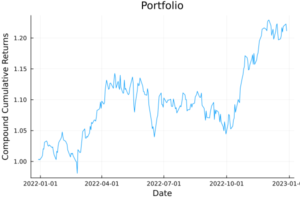
The plot of each asset's risk contribution needs a risk measure with its statistics set, here the covariance matrix of a Variance. factory builds a copy of the measure that takes its covariance from the prior result res.pr. You can also set it by hand, but factory is the better choice in code that builds many measures.
The risk measure needs this step because the library keeps the risk measures apart from the optimisers and their results. The same design lets you put several risk measures in one objective, or use a risk measure as a limit in an optimisation. The examples show both.
plot_risk_contribution(factory(Variance(), res.pr), mip_res.w, rd.X; nx = rd.nx)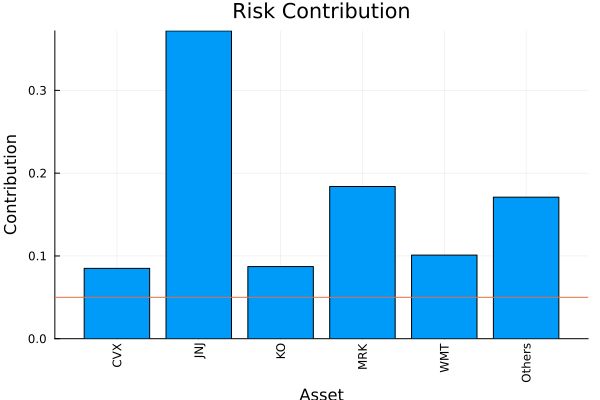
The histogram shows the distribution of the portfolio returns.
plot_histogram(mip_res.w, rd.X; slv = slv)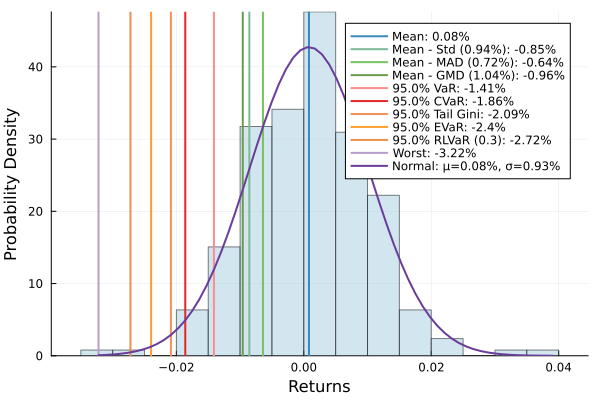
The drawdown plot shows the compounded drawdowns. Pass compound = false for the uncompounded ones.
plot_drawdowns(mip_res.w, rd.X; slv = slv, ts = rd.ts, compound = true)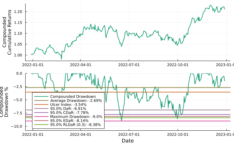
The Plotting page lists the other plots.