The source files can be found in user_guide/.
Optimisers
This is the breadth tour of the optimiser families. Every optimiser shares the same call — optimise(estimator) (or optimise(estimator, rd) for the naive and meta ones) — and returns a result whose w field holds the asset weights. The point of this page is to show the shape of each family with one minimal call; for objectives, risk measures, variants, and trade-offs, follow the cross-links into the optimiser examples.
We fix one empirical prior and reuse it everywhere so the families are comparable.
using PortfolioOptimisers, CSV, TimeSeries, DataFrames, PrettyTables, Clarabel, StatsPlots, GraphRecipesresfmt = (v, i, j) -> begin return if j == 1 v else isa(v, AbstractFloat) ? "$(round(v*100, digits=3)) %" : v endend;X = TimeArray(CSV.File(joinpath(@__DIR__, "../examples/SP500.csv.gz")); timestamp = :Date)[(end - 252):end]rd = prices_to_returns(X)pr = prior(EmpiricalPrior(), rd)LowOrderPrior
X ┼ 252×20 Matrix{Float64}
o_X ┼ nothing
mu ┼ 20-element Vector{Float64}
sigma ┼ 20×20 Matrix{Float64}
chol ┼ nothing
w ┼ nothing
ens ┼ nothing
kld ┼ nothing
ow ┼ nothing
rr ┼ nothing
fpr ┼ nothing
Z ┴ nothing
Every JuMP optimiser below shares this one solver. Its check_sol field is splatted into JuMP's assert_is_solved_and_feasible after each solve, and decides which solver statuses count as a solved model. The default (;) is strict on purpose — it accepts only OPTIMAL or LOCALLY_SOLVED at a FEASIBLE_POINT, so a solution the solver itself flags as approximate is rejected rather than silently used. Passing allow_almost = true widens it to the ALMOST_* statuses, which is what we want here: a first-order conic solver that reaches its tolerance on a well-posed portfolio problem gives a usable answer, and rejecting it would only make the optimiser fall through to the next solver. Tighten it the other way with allow_local = false when nothing short of a certified global optimum will do.
slv = Solver(; name = :clarabel, solver = Clarabel.Optimizer, settings = Dict("verbose" => false), check_sol = (; allow_local = true, allow_almost = true))Solver
name ┼ Symbol: :clarabel
solver ┼ UnionAll: Clarabel.MOIwrapper.Optimizer
settings ┼ Dict{String, Bool}: Dict{String, Bool}("verbose" => 0)
check_sol ┼ @NamedTuple{allow_local::Bool, allow_almost::Bool}: (allow_local = true, allow_almost = true)
add_bridges ┴ Bool: true
1. Naive optimisers
Naive optimisers use simple, solver-free rules that buy robustness through unsophistication. InverseVolatility weights by the reciprocal of each asset's volatility; EqualWeighted splits capital evenly; RandomWeighted samples a Dirichlet allocation. They take the ReturnsResult directly.
res_iv = optimise(InverseVolatility(), rd)res_ew = optimise(EqualWeighted(), rd)NaiveOptimisationResult
pr ┼ ReturnsResult
│ nx ┼ 20-element Vector{String}
│ X ┼ 252×20 Matrix{Float64}
│ nf ┼ nothing
│ F ┼ nothing
│ nb ┼ nothing
│ B ┼ nothing
│ ts ┼ 252-element Vector{Date}
│ iv ┼ nothing
│ ivpa ┼ nothing
│ nz ┼ nothing
│ Z ┴ nothing
wb ┼ WeightBounds
│ lb ┼ 20-element StepRangeLen{Float64, Base.TwicePrecision{Float64}, Base.TwicePrecision{Float64}, Int64}
│ ub ┴ 20-element StepRangeLen{Float64, Base.TwicePrecision{Float64}, Base.TwicePrecision{Float64}, Int64}
retcode ┼ OptimisationSuccess
│ res ┴ nothing
w ┼ 20-element Vector{Float64}
fb ┴ nothing
2. JuMP optimisers — MeanRisk
JuMP optimisers solve a mathematical program and are the most flexible on constraints, objectives, and risk measures. They need a JuMPOptimiser carrying the prior and a Solver (we recommend Clarabel for non-MIP problems). The workhorse is MeanRisk; its default objective is MinimumRisk.
res_mr = optimise(MeanRisk(; obj = MinimumRisk(), opt = JuMPOptimiser(; pe = pr, slv = slv)))MeanRiskResult
jr ┼ JuMPOptimisationResult
│ pa ┼ ProcessedJuMPOptimiserAttributes
│ │ pr ┼ LowOrderPrior
│ │ │ X ┼ 252×20 Matrix{Float64}
│ │ │ o_X ┼ nothing
│ │ │ mu ┼ 20-element Vector{Float64}
│ │ │ sigma ┼ 20×20 Matrix{Float64}
│ │ │ chol ┼ nothing
│ │ │ w ┼ nothing
│ │ │ ens ┼ nothing
│ │ │ kld ┼ nothing
│ │ │ ow ┼ nothing
│ │ │ rr ┼ nothing
│ │ │ fpr ┼ nothing
│ │ │ Z ┴ nothing
│ │ wb ┼ WeightBounds
│ │ │ lb ┼ 20-element StepRangeLen{Float64, Base.TwicePrecision{Float64}, Base.TwicePrecision{Float64}, Int64}
│ │ │ ub ┴ 20-element StepRangeLen{Float64, Base.TwicePrecision{Float64}, Base.TwicePrecision{Float64}, Int64}
│ │ lt ┼ nothing
│ │ st ┼ nothing
│ │ lcsr ┼ nothing
│ │ ctr ┼ nothing
│ │ gcardr ┼ nothing
│ │ sgcardr ┼ nothing
│ │ smtx ┼ nothing
│ │ sgmtx ┼ nothing
│ │ slt ┼ nothing
│ │ sst ┼ nothing
│ │ sglt ┼ nothing
│ │ sgst ┼ nothing
│ │ tn ┼ nothing
│ │ fees ┼ nothing
│ │ plr ┼ nothing
│ │ ret ┼ ArithmeticReturn
│ │ │ settings ┼ JuMPReturnsSettings
│ │ │ │ scale ┼ Float64: 1.0
│ │ │ │ lb ┼ nothing
│ │ │ │ rte ┼ Bool: true
│ │ │ │ fee ┼ Bool: true
│ │ │ │ mic ┴ Bool: true
│ │ │ ucs ┼ nothing
│ │ │ mu ┴ 20-element Vector{Float64}
│ │ sca ┴ SumScalariser()
│ retcode ┼ OptimisationSuccess
│ │ res ┴ Dict{Any, Any}: Dict{Any, Any}()
│ sol ┼ JuMPOptimisationSolution
│ │ w ┴ 20-element Vector{Float64}
│ model ┼ A JuMP Model
│ │ ├ solver: Clarabel
│ │ ├ objective_sense: MIN_SENSE
│ │ │ └ objective_function_type: QuadExpr
│ │ ├ num_variables: 21
│ │ ├ num_constraints: 4
│ │ │ ├ AffExpr in MOI.EqualTo{Float64}: 1
│ │ │ ├ Vector{AffExpr} in MOI.Nonnegatives: 1
│ │ │ ├ Vector{AffExpr} in MOI.Nonpositives: 1
│ │ │ └ Vector{AffExpr} in MOI.SecondOrderCone: 1
│ │ └ Names registered in the model
│ │ └ :G, :bgt, :cdev_soc_1, :dev_1, :k, :lw, :obj_expr, :ret, :ret_1, :ret_vec, :risk, :risk_vec, :sc, :so, :variance_flag, :variance_risk_1, :w, :w_lb, :w_ub
r ┼ Variance
│ settings ┼ RiskMeasureSettings
│ │ scale ┼ Float64: 1.0
│ │ ub ┼ nothing
│ │ rke ┴ Bool: true
│ sigma ┼ 20×20 Matrix{Float64}
│ chol ┼ nothing
│ rc ┼ nothing
│ alg ┴ SquaredSOCRiskExpr()
fb ┴ nothing
MeanRisk also offers MaximumUtility, MaximumRatio and MaximumReturn objectives and efficient frontiers — see MeanRisk Objectives and Efficient Frontier.
The risk measure is the r field (of MeanRisk and of the clustering optimisers below); the default is Variance. Which one you pick encodes what kind of risk you penalise — overall dispersion (Variance), the left tail (ConditionalValueatRisk), peak-to-trough paths (MaximumDrawdown), or the whole ordered loss curve (OrderedWeightsArray). The full menu — every measure with its alias, its meaning, and which optimisers accept it — is the risk measures page; you can also mix several in one objective (Multiple Risk Measures).
The return side is the ret field of JuMPOptimiser, an ArithmeticReturn by default. Like r, it takes one term or a vector of them, summed with weights into the model's single return expression. Each term carries its own JuMPReturnsSettings — its weight in that sum, its own lower bound, and whether it enters the sum at all — so a term can bound the portfolio without being rewarded, which is how you price what a floor on one quantity costs in another (ℓ1 uncertainty sets).
The drawdown notion is also useful purely as a post-optimisation diagnostic — via drawdowns on a realised book — when you want to measure rather than optimise it (Performance Attribution).
The other JuMP families follow the same opt = JuMPOptimiser(...) pattern:
RiskBudgeting/RelaxedRiskBudgeting— target a risk contribution per asset or factor (Risk Budgeting).NearOptimalCentering— a robust point near the efficient frontier (Near Optimal Centering).
Here is the minimal risk-budgeting call (equal risk contribution by default):
res_rb = optimise(RiskBudgeting(; opt = JuMPOptimiser(; pe = pr, slv = slv)))RiskBudgetingResult
jr ┼ JuMPOptimisationResult
│ pa ┼ ProcessedJuMPOptimiserAttributes
│ │ pr ┼ LowOrderPrior
│ │ │ X ┼ 252×20 Matrix{Float64}
│ │ │ o_X ┼ nothing
│ │ │ mu ┼ 20-element Vector{Float64}
│ │ │ sigma ┼ 20×20 Matrix{Float64}
│ │ │ chol ┼ nothing
│ │ │ w ┼ nothing
│ │ │ ens ┼ nothing
│ │ │ kld ┼ nothing
│ │ │ ow ┼ nothing
│ │ │ rr ┼ nothing
│ │ │ fpr ┼ nothing
│ │ │ Z ┴ nothing
│ │ wb ┼ WeightBounds
│ │ │ lb ┼ 20-element StepRangeLen{Float64, Base.TwicePrecision{Float64}, Base.TwicePrecision{Float64}, Int64}
│ │ │ ub ┴ 20-element StepRangeLen{Float64, Base.TwicePrecision{Float64}, Base.TwicePrecision{Float64}, Int64}
│ │ lt ┼ nothing
│ │ st ┼ nothing
│ │ lcsr ┼ nothing
│ │ ctr ┼ nothing
│ │ gcardr ┼ nothing
│ │ sgcardr ┼ nothing
│ │ smtx ┼ nothing
│ │ sgmtx ┼ nothing
│ │ slt ┼ nothing
│ │ sst ┼ nothing
│ │ sglt ┼ nothing
│ │ sgst ┼ nothing
│ │ tn ┼ nothing
│ │ fees ┼ nothing
│ │ plr ┼ nothing
│ │ ret ┼ ArithmeticReturn
│ │ │ settings ┼ JuMPReturnsSettings
│ │ │ │ scale ┼ Float64: 1.0
│ │ │ │ lb ┼ nothing
│ │ │ │ rte ┼ Bool: true
│ │ │ │ fee ┼ Bool: true
│ │ │ │ mic ┴ Bool: true
│ │ │ ucs ┼ nothing
│ │ │ mu ┴ 20-element Vector{Float64}
│ │ sca ┴ SumScalariser()
│ retcode ┼ OptimisationSuccess
│ │ res ┴ Dict{Any, Any}: Dict{Any, Any}()
│ sol ┼ JuMPOptimisationSolution
│ │ w ┴ 20-element Vector{Float64}
│ model ┼ A JuMP Model
│ │ ├ solver: Clarabel
│ │ ├ objective_sense: MIN_SENSE
│ │ │ └ objective_function_type: QuadExpr
│ │ ├ num_variables: 42
│ │ ├ num_constraints: 25
│ │ │ ├ AffExpr in MOI.EqualTo{Float64}: 1
│ │ │ ├ AffExpr in MOI.GreaterThan{Float64}: 1
│ │ │ ├ Vector{AffExpr} in MOI.Nonnegatives: 1
│ │ │ ├ Vector{AffExpr} in MOI.Nonpositives: 1
│ │ │ ├ Vector{AffExpr} in MOI.SecondOrderCone: 1
│ │ │ └ Vector{AffExpr} in MOI.ExponentialCone: 20
│ │ └ Names registered in the model
│ │ └ :G, :bgt, :cdev_soc_1, :clog_w, :crkb, :dev_1, :k, :log_w, :lw, :obj_expr, :ret, :ret_1, :ret_vec, :risk, :risk_vec, :sc, :so, :unit_budget, :variance_flag, :variance_risk_1, :w, :w_lb, :w_ub
r ┼ Variance
│ settings ┼ RiskMeasureSettings
│ │ scale ┼ Float64: 1.0
│ │ ub ┼ nothing
│ │ rke ┴ Bool: true
│ sigma ┼ 20×20 Matrix{Float64}
│ chol ┼ nothing
│ rc ┼ nothing
│ alg ┴ SquaredSOCRiskExpr()
prb ┼ ProcessedAssetRiskBudgetingAttributes
│ rkb ┼ RiskBudget
│ │ val ┴ 20-element StepRangeLen{Float64, Base.TwicePrecision{Float64}, Base.TwicePrecision{Float64}, Int64}
fb ┴ nothing
Which risk measures each optimiser family accepts
Compatibility is a property of the optimiser family, not the individual optimiser: every JuMP optimiser accepts the same RiskMeasures, and clustering optimisers additionally accept the hierarchical-only measures. You can ask programmatically with supports_risk_measure / supported_risk_measures:
supports_risk_measure(MeanRisk, ConditionalValueatRisk) # truesupported_risk_measures(HierarchicalRiskParity) # OptimisationRiskMeasureMeta-optimisers (NestedClustered, Stacking, SubsetResampling) are the exception: their acceptance is instance-specific because they delegate, accepting a measure only when every constituent optimiser does (the intersection of their children's categories).
The risk measures page tabulates every measure against these classes — the tables there are generated from the same predicate, so they cannot drift from what the optimisers actually dispatch on.
3. Clustering optimisers
Clustering optimisers build the allocation from the asset correlation hierarchy instead of a single program. They take a HierarchicalOptimiser carrying the prior and a clustering estimate. HierarchicalRiskParity (HRP) is the canonical one; HierarchicalEqualRiskContribution and SchurComplementHierarchicalRiskParity are its siblings — see Clustering Optimisers.
clr = clusterise(ClustersEstimator(), pr.X)hopt = HierarchicalOptimiser(; pe = pr, cle = clr)res_hrp = optimise(HierarchicalRiskParity(; opt = hopt, r = Variance()))HierarchicalRiskParityResult
hr ┼ HierarchicalResult
│ pr ┼ LowOrderPrior
│ │ X ┼ 252×20 Matrix{Float64}
│ │ o_X ┼ nothing
│ │ mu ┼ 20-element Vector{Float64}
│ │ sigma ┼ 20×20 Matrix{Float64}
│ │ chol ┼ nothing
│ │ w ┼ nothing
│ │ ens ┼ nothing
│ │ kld ┼ nothing
│ │ ow ┼ nothing
│ │ rr ┼ nothing
│ │ fpr ┼ nothing
│ │ Z ┴ nothing
│ clr ┼ Clusters
│ │ res ┼ Clustering.Hclust{Float64}([-1 -13; -2 1; … ; 15 16; 18 17], [0.2992796916890263, 0.39056120313611004, 0.4116454947407609, 0.22529867864314176, 0.48924055164900887, 0.28518628966607656, 0.3800863165339249, 0.5842580180890099, 0.4209146698909511, 0.4605479608276049, 0.491265779899127, 0.5080236207888611, 0.6028393326616824, 0.24670816017739164, 0.5174631833197462, 0.6821605083740293, 0.7399456049755042, 0.9602133336085281, 1.07073891752418], [5, 20, 17, 3, 9, 6, 2, 1, 13, 7, 4, 19, 14, 10, 16, 18, 11, 8, 12, 15], :ward)
│ │ S ┼ 20×20 Matrix{Float64}
│ │ D ┼ 20×20 Matrix{Float64}
│ │ P ┼ nothing
│ │ k ┴ Int64: 2
│ wb ┼ WeightBounds
│ │ lb ┼ 20-element StepRangeLen{Float64, Base.TwicePrecision{Float64}, Base.TwicePrecision{Float64}, Int64}
│ │ ub ┴ 20-element StepRangeLen{Float64, Base.TwicePrecision{Float64}, Base.TwicePrecision{Float64}, Int64}
│ fees ┼ nothing
│ retcode ┼ OptimisationSuccess
│ │ res ┴ nothing
│ w ┴ 20-element Vector{Float64}
r ┼ Variance
│ settings ┼ RiskMeasureSettings
│ │ scale ┼ Float64: 1.0
│ │ ub ┼ nothing
│ │ rke ┴ Bool: true
│ sigma ┼ 20×20 Matrix{Float64}
│ chol ┼ nothing
│ rc ┼ nothing
│ alg ┴ SquaredSOCRiskExpr()
sca ┼ SumScalariser()
fb ┴ nothing
3.1 Clustering on something other than the returns
clusterise(ClustersEstimator(), pr.X) derives its distance from the correlation, so the hierarchy can only ever see structure the price history contains. Swapping the estimator's distance slot for a FeatureDistance clusters an assets × features matrix instead — a sector or country classification, a factor loading profile, any per-asset quantity you can name. asset_sets_features builds one from a UniverseSets taxonomy, and it travels beside the returns as data rather than on the estimator.
sector = Dict("AAPL" => "Tech", "AMD" => "Tech", "MSFT" => "Tech", "BAC" => "Financials", "JPM" => "Financials", "CVX" => "Energy", "XOM" => "Energy", "RRC" => "Energy", "GE" => "Industrials", "BBY" => "Discretionary", "HD" => "Discretionary", "KO" => "Staples", "PEP" => "Staples", "PG" => "Staples", "WMT" => "Staples", "JNJ" => "Health", "LLY" => "Health", "MRK" => "Health", "PFE" => "Health", "UNH" => "Health")revenue = Dict("AAPL" => "Global", "AMD" => "Global", "MSFT" => "Global", "BAC" => "Domestic", "JPM" => "Global", "CVX" => "Global", "XOM" => "Global", "RRC" => "Domestic", "GE" => "Global", "BBY" => "Domestic", "HD" => "Domestic", "KO" => "Global", "PEP" => "Global", "PG" => "Global", "WMT" => "Domestic", "JNJ" => "Global", "LLY" => "Global", "MRK" => "Global", "PFE" => "Global", "UNH" => "Domestic")sets_z = UniverseSets(; xkey = "nx", dict = Dict("nx" => rd.nx, "nx_sector" => [sector[a] for a in rd.nx], "nx_revenue" => [revenue[a] for a in rd.nx]))vals_z = ["nx_sector", "nx_revenue"]rd_z = ReturnsResult(; nx = rd.nx, X = rd.X, ts = rd.ts, nz = asset_sets_feature_names(vals_z, sets_z), Z = asset_sets_features(vals_z, sets_z))res_hrp_z = optimise(HierarchicalRiskParity(; opt = HierarchicalOptimiser(; pe = pr, cle = ClustersEstimator(; de = FeatureDistance()), z_src = :data), r = Variance()), rd_z)HierarchicalRiskParityResult
hr ┼ HierarchicalResult
│ pr ┼ LowOrderPrior
│ │ X ┼ 252×20 Matrix{Float64}
│ │ o_X ┼ nothing
│ │ mu ┼ 20-element Vector{Float64}
│ │ sigma ┼ 20×20 Matrix{Float64}
│ │ chol ┼ nothing
│ │ w ┼ nothing
│ │ ens ┼ nothing
│ │ kld ┼ nothing
│ │ ow ┼ nothing
│ │ rr ┼ nothing
│ │ fpr ┼ nothing
│ │ Z ┴ nothing
│ clr ┼ Clusters
│ │ res ┼ Clustering.Hclust{Float64}([-1 -2; 1 -13; … ; 5 15; 17 18], [6.707879276254074e-9, 6.707879276254074e-9, 6.707879276254074e-9, 6.707879276254074e-9, 6.707879276254074e-9, 0.33333333333333337, 6.707879276254074e-9, 0.33333333333333337, 6.707879276254074e-9, 6.707879276254074e-9, 6.707879276254074e-9, 0.33333333333333337, 0.408248290463863, 0.511766315719159, 0.33333333333333337, 0.5520524474738834, 0.6274159654095468, 0.43033148291193524, 1.1075737342134728], [1, 2, 13, 20, 5, 6, 9, 16, 14, 10, 15, 8, 11, 12, 4, 7, 3, 18, 17, 19], :ward)
│ │ S ┼ 20×20 Matrix{Float64}
│ │ D ┼ 20×20 Matrix{Float64}
│ │ P ┼ nothing
│ │ k ┴ Int64: 3
│ wb ┼ WeightBounds
│ │ lb ┼ 20-element StepRangeLen{Float64, Base.TwicePrecision{Float64}, Base.TwicePrecision{Float64}, Int64}
│ │ ub ┴ 20-element StepRangeLen{Float64, Base.TwicePrecision{Float64}, Base.TwicePrecision{Float64}, Int64}
│ fees ┼ nothing
│ retcode ┼ OptimisationSuccess
│ │ res ┴ nothing
│ w ┴ 20-element Vector{Float64}
r ┼ Variance
│ settings ┼ RiskMeasureSettings
│ │ scale ┼ Float64: 1.0
│ │ ub ┼ nothing
│ │ rke ┴ Bool: true
│ sigma ┼ 20×20 Matrix{Float64}
│ chol ┼ nothing
│ rc ┼ nothing
│ alg ┴ SquaredSOCRiskExpr()
sca ┼ SumScalariser()
fb ┴ nothing
z_src picks which of the two carriers supplies the matrix: :data reads the one you supplied on the ReturnsResult, :prior reads one a producer derived onto the prior result. It defaults to :data — the opposite of x_src — because an explicitly supplied matrix outranks a derived one.
Two consequences only appear once cross-validation is switched on, and neither can be inferred from the API:
:dataslices,:priorrefits. Inside a fold or a meta-optimiser's subproblem, a carried matrix is subselected while a derived one is recomputed on the subproblem's own returns. For a fixed classification the two coincide; for a returns-derived producer they are two different questions, so the selector chooses between two semantics rather than two copies.- A time-varying literal matrix cannot survive an observation fold. A three-dimensional
observations × assets × featuresmatrix handed straight toFeaturePriorhas no way to be resliced down its observation axis, so the fit throws aDimensionMismatchas soon as the observation count changes. Features that must vary with time and survive folds have to come from a producer, which refits on whatever rows the fold hands it.
See Feature Matrices as a Distance Source for the four producers, the time-varying shapes, and a walk-forward comparison.
4. Meta-optimisers
Meta-optimisers compose other optimisers. NestedClustered (NCO) runs an inner optimiser within each cluster and an outer optimiser across the cluster representatives; Stacking and SubsetResampling blend several fits — see Meta Optimisers. The inner optimiser carries the prior; the outer one does not.
res_nco = optimise(NestedClustered(; pe = pr, cle = clr, opti = MeanRisk(; obj = MinimumRisk(), opt = JuMPOptimiser(; pe = pr, slv = slv)), opto = MeanRisk(; obj = MinimumRisk(), opt = JuMPOptimiser(; slv = slv))), rd)NestedClusteredResult
pr ┼ LowOrderPrior
│ X ┼ 252×20 Matrix{Float64}
│ o_X ┼ nothing
│ mu ┼ 20-element Vector{Float64}
│ sigma ┼ 20×20 Matrix{Float64}
│ chol ┼ nothing
│ w ┼ nothing
│ ens ┼ nothing
│ kld ┼ nothing
│ ow ┼ nothing
│ rr ┼ nothing
│ fpr ┼ nothing
│ Z ┴ nothing
clr ┼ Clusters
│ res ┼ Clustering.Hclust{Float64}([-1 -13; -2 1; … ; 15 16; 18 17], [0.2992796916890263, 0.39056120313611004, 0.4116454947407609, 0.22529867864314176, 0.48924055164900887, 0.28518628966607656, 0.3800863165339249, 0.5842580180890099, 0.4209146698909511, 0.4605479608276049, 0.491265779899127, 0.5080236207888611, 0.6028393326616824, 0.24670816017739164, 0.5174631833197462, 0.6821605083740293, 0.7399456049755042, 0.9602133336085281, 1.07073891752418], [5, 20, 17, 3, 9, 6, 2, 1, 13, 7, 4, 19, 14, 10, 16, 18, 11, 8, 12, 15], :ward)
│ S ┼ 20×20 Matrix{Float64}
│ D ┼ 20×20 Matrix{Float64}
│ P ┼ nothing
│ k ┴ Int64: 2
wb ┼ WeightBounds
│ lb ┼ 20-element Vector{Float64}
│ ub ┴ 20-element Vector{Float64}
fees ┼ nothing
resi ┼ 2-element Vector{MeanRiskResult}
│ MeanRiskResult ⋯
│ MeanRiskResult ⋯
reso ┼ MeanRiskResult
│ jr ┼ JuMPOptimisationResult
│ │ pa ┼ ProcessedJuMPOptimiserAttributes
│ │ │ pr ┼ LowOrderPrior
│ │ │ │ X ┼ 252×2 Matrix{Float64}
│ │ │ │ o_X ┼ nothing
│ │ │ │ mu ┼ Vector{Float64}: [0.00036354628076020715, 0.000652797420571548]
│ │ │ │ sigma ┼ 2×2 Matrix{Float64}
│ │ │ │ chol ┼ nothing
│ │ │ │ w ┼ nothing
│ │ │ │ ens ┼ nothing
│ │ │ │ kld ┼ nothing
│ │ │ │ ow ┼ nothing
│ │ │ │ rr ┼ nothing
│ │ │ │ fpr ┼ nothing
│ │ │ │ Z ┴ nothing
│ │ │ wb ┼ WeightBounds
│ │ │ │ lb ┼ StepRangeLen{Float64, Base.TwicePrecision{Float64}, Base.TwicePrecision{Float64}, Int64}: StepRangeLen(0.0, 0.0, 2)
│ │ │ │ ub ┴ StepRangeLen{Float64, Base.TwicePrecision{Float64}, Base.TwicePrecision{Float64}, Int64}: StepRangeLen(1.0, 0.0, 2)
│ │ │ lt ┼ nothing
│ │ │ st ┼ nothing
│ │ │ lcsr ┼ nothing
│ │ │ ctr ┼ nothing
│ │ │ gcardr ┼ nothing
│ │ │ sgcardr ┼ nothing
│ │ │ smtx ┼ nothing
│ │ │ sgmtx ┼ nothing
│ │ │ slt ┼ nothing
│ │ │ sst ┼ nothing
│ │ │ sglt ┼ nothing
│ │ │ sgst ┼ nothing
│ │ │ tn ┼ nothing
│ │ │ fees ┼ nothing
│ │ │ plr ┼ nothing
│ │ │ ret ┼ ArithmeticReturn
│ │ │ │ settings ┼ JuMPReturnsSettings
│ │ │ │ │ scale ┼ Float64: 1.0
│ │ │ │ │ lb ┼ nothing
│ │ │ │ │ rte ┼ Bool: true
│ │ │ │ │ fee ┼ Bool: true
│ │ │ │ │ mic ┴ Bool: true
│ │ │ │ ucs ┼ nothing
│ │ │ │ mu ┴ Vector{Float64}: [0.00036354628076020715, 0.000652797420571548]
│ │ │ sca ┴ SumScalariser()
│ │ retcode ┼ OptimisationSuccess
│ │ │ res ┴ Dict{Any, Any}: Dict{Any, Any}()
│ │ sol ┼ JuMPOptimisationSolution
│ │ │ w ┴ Vector{Float64}: [0.13998673390958633, 0.8600132660904137]
│ │ model ┼ A JuMP Model
│ │ │ ├ solver: Clarabel
│ │ │ ├ objective_sense: MIN_SENSE
│ │ │ │ └ objective_function_type: QuadExpr
│ │ │ ├ num_variables: 3
│ │ │ ├ num_constraints: 4
│ │ │ │ ├ AffExpr in MOI.EqualTo{Float64}: 1
│ │ │ │ ├ Vector{AffExpr} in MOI.Nonnegatives: 1
│ │ │ │ ├ Vector{AffExpr} in MOI.Nonpositives: 1
│ │ │ │ └ Vector{AffExpr} in MOI.SecondOrderCone: 1
│ │ │ └ Names registered in the model
│ │ │ └ :G, :bgt, :cdev_soc_1, :dev_1, :k, :lw, :obj_expr, :ret, :ret_1, :ret_vec, :risk, :risk_vec, :sc, :so, :variance_flag, :variance_risk_1, :w, :w_lb, :w_ub
│ r ┼ Variance
│ │ settings ┼ RiskMeasureSettings
│ │ │ scale ┼ Float64: 1.0
│ │ │ ub ┼ nothing
│ │ │ rke ┴ Bool: true
│ │ sigma ┼ 2×2 Matrix{Float64}
│ │ chol ┼ nothing
│ │ rc ┼ nothing
│ │ alg ┴ SquaredSOCRiskExpr()
│ fb ┴ nothing
cv ┼ nothing
retcode ┼ OptimisationSuccess
│ res ┴ nothing
w ┼ 20-element Vector{Float64}
fb ┴ nothing
5. Comparing the families
One prior, six optimisers, six allocations. The naive rules, risk budgeting, and the clustering hierarchy spread weight broadly (max weight in single digits to low teens); MeanRisk(MinimumRisk) and NCO concentrate into a few low-variance names (max weight ≈ a third). Same data, very different portfolios — which is the point of having a menu.
results = [res_iv, res_ew, res_mr, res_rb, res_hrp, res_nco]labels = ["InvVol", "EqualW", "MinRisk", "RiskBudget", "HRP", "NCO"]pretty_table(DataFrame(["Asset" => rd.nx, [labels[i] => results[i].w for i in eachindex(results)]...]); formatters = [resfmt], title = "Weights by optimiser family")plot_stacked_bar_composition(results, rd; xticks = (1:length(labels), labels))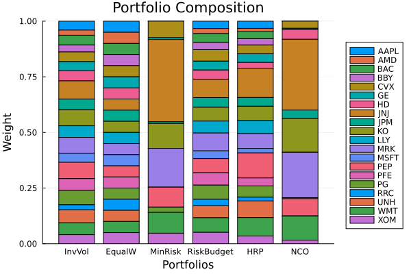
This page was generated using Literate.jl.