The source files can be found in examples/.
Getting started: a simple MeanRisk optimisation
This page runs the classic Markowitz optimisation with PortfolioOptimisers, from a table of prices to a portfolio you can buy with a fixed amount of cash.
using PortfolioOptimisersWe use PrettyTables to format the tables the page prints.
using PrettyTablestsfmt = (v, i, j) -> begin if j == 1 return Date(v) else return v endend;resfmt = (v, i, j) -> begin if j == 1 return v else return isa(v, Number) ? "$(round(v*100, digits=3)) %" : v endend;mipresfmt = (v, i, j) -> begin if j ∈ (1, 2, 3) return v else return isa(v, Number) ? "$(round(v*100, digits=3)) %" : v endend;1. Load the data
We load the S&P 500 prices from a compressed .csv file and keep the last 253 observations.
using CSV, TimeSeries, DataFramesX = TimeArray(CSV.File(joinpath(@__DIR__, "..", "SP500.csv.gz")); timestamp = :Date)[(end - 252):end]pretty_table(X[(end - 5):end]; formatters = [tsfmt])┌────────────┬─────────┬─────────┬─────────┬─────────┬─────────┬─────────┬─────────┬─────────┬─────────┬─────────┬─────────┬─────────┬─────────┬─────────┬─────────┬─────────┬─────────┬─────────┬─────────┬─────────┐
│ timestamp │ AAPL │ AMD │ BAC │ BBY │ CVX │ GE │ HD │ JNJ │ JPM │ KO │ LLY │ MRK │ MSFT │ PEP │ PFE │ PG │ RRC │ UNH │ WMT │ XOM │
│ Date │ Float64 │ Float64 │ Float64 │ Float64 │ Float64 │ Float64 │ Float64 │ Float64 │ Float64 │ Float64 │ Float64 │ Float64 │ Float64 │ Float64 │ Float64 │ Float64 │ Float64 │ Float64 │ Float64 │ Float64 │
├────────────┼─────────┼─────────┼─────────┼─────────┼─────────┼─────────┼─────────┼─────────┼─────────┼─────────┼─────────┼─────────┼─────────┼─────────┼─────────┼─────────┼─────────┼─────────┼─────────┼─────────┤
│ 2022-12-20 │ 131.916 │ 65.05 │ 31.729 │ 77.371 │ 169.497 │ 62.604 │ 310.342 │ 173.109 │ 127.844 │ 61.841 │ 357.55 │ 108.229 │ 240.67 │ 178.765 │ 49.754 │ 147.661 │ 25.65 │ 516.245 │ 142.919 │ 104.964 │
│ 2022-12-21 │ 135.057 │ 67.68 │ 32.212 │ 78.729 │ 171.49 │ 64.67 │ 314.798 │ 175.09 │ 129.282 │ 62.836 │ 365.872 │ 109.611 │ 243.287 │ 180.017 │ 50.084 │ 149.015 │ 26.574 │ 523.519 │ 144.04 │ 106.312 │
│ 2022-12-22 │ 131.846 │ 63.86 │ 31.927 │ 78.563 │ 168.918 │ 63.727 │ 311.604 │ 174.45 │ 127.814 │ 62.383 │ 363.187 │ 109.739 │ 237.077 │ 178.627 │ 50.065 │ 149.359 │ 25.232 │ 523.072 │ 142.354 │ 104.168 │
│ 2022-12-23 │ 131.477 │ 64.52 │ 32.005 │ 79.432 │ 174.14 │ 63.742 │ 314.177 │ 174.893 │ 128.421 │ 62.855 │ 365.762 │ 110.35 │ 237.614 │ 179.781 │ 50.249 │ 149.781 │ 26.226 │ 527.26 │ 142.641 │ 106.922 │
│ 2022-12-27 │ 129.652 │ 63.27 │ 32.065 │ 79.93 │ 176.329 │ 64.561 │ 314.985 │ 174.844 │ 128.871 │ 63.24 │ 362.76 │ 110.607 │ 235.852 │ 180.58 │ 49.57 │ 151.086 │ 26.375 │ 527.935 │ 142.681 │ 108.408 │
│ 2022-12-28 │ 125.674 │ 62.57 │ 32.301 │ 78.279 │ 173.728 │ 63.883 │ 311.22 │ 174.085 │ 129.575 │ 62.609 │ 363.098 │ 109.581 │ 233.434 │ 179.278 │ 49.25 │ 149.133 │ 24.497 │ 524.422 │ 140.181 │ 106.627 │
└────────────┴─────────┴─────────┴─────────┴─────────┴─────────┴─────────┴─────────┴─────────┴─────────┴─────────┴─────────┴─────────┴─────────┴─────────┴─────────┴─────────┴─────────┴─────────┴─────────┴─────────┘The optimiser works on returns, so we compute them from the prices. The ReturnsResult that comes back stores the asset names in nx, the asset returns in X and the timestamps in ts. Its other fields store data that this page does not use.
rd = prices_to_returns(X)ReturnsResult
nx ┼ 20-element Vector{String}
X ┼ 252×20 Matrix{Float64}
nf ┼ nothing
F ┼ nothing
nb ┼ nothing
B ┼ nothing
ne ┼ nothing
E ┼ nothing
ts ┼ 252-element Vector{Date}
iv ┼ nothing
ivpa ┼ nothing
pnl ┼ AssetPanel
│ pf ┼ Vector{AbstractPanelField}: AbstractPanelField[]
│ amsk ┼ 252×20 AllTrueMask
│ emsk ┴ 252×20 AllTrueMask
2. MeanRisk optimisation
2.1 Creating a solver instance
Every optimisation needs statistics of the returns, such as their mean and covariance, which the library calls the prior. You can compute the prior before the optimisation and pass it in, or let the optimisation compute it. Computing it first saves time when several optimisations share one prior. Here there is only one optimisation, so we let it compute its own.
The MeanRisk estimator states a mean-risk optimisation problem. The library builds that problem as a JuMP model, so MeanRisk needs a solver that JuMP can call. We use Clarabel.
using ClarabelA Solver takes the solver to use, an optional name that appears in the logs, optional solver settings, and optional keyword arguments for JuMP.assert_is_solved_and_feasible.
A hard problem can fail with one solver or one group of settings and succeed with another. For that case you can pass a vector of Solver objects, and the optimisation tries each in turn until one succeeds or all fail. The Markowitz problem is easy to solve, so we use one solver.
slv = Solver(; name = :clarabel1, solver = Clarabel.Optimizer, settings = Dict("verbose" => false), check_sol = (; allow_local = true, allow_almost = true))Solver
name ┼ Symbol: :clarabel1
solver ┼ UnionAll: Clarabel.MOIwrapper.Optimizer
settings ┼ Dict{String, Bool}: Dict{String, Bool}("verbose" => 0)
check_sol ┼ @NamedTuple{allow_local::Bool, allow_almost::Bool}: (allow_local = true, allow_almost = true)
add_bridges ┴ Bool: true
2.2 Defining the optimisation estimator
PortfolioOptimisers builds an optimisation out of smaller estimators. MeanRisk takes its solver, its constraints and its prior estimator from a JuMPOptimiser, in its opt field.
We create a MeanRisk estimator. The printed output lists many more fields of JuMPOptimiser and MeanRisk than this page uses.
mr = MeanRisk(; opt = JuMPOptimiser(; slv = slv))MeanRisk
opt ┼ JuMPOptimiser
│ pe ┼ EmpiricalPrior
│ │ ce ┼ PortfolioOptimisersCovariance
│ │ │ ce ┼ Covariance
│ │ │ │ me ┼ SimpleExpectedReturns
│ │ │ │ │ w ┴ nothing
│ │ │ │ ce ┼ GeneralCovariance
│ │ │ │ │ ce ┼ SimpleCovariance: SimpleCovariance(true)
│ │ │ │ │ w ┴ nothing
│ │ │ │ alg ┼ FullMoment()
│ │ │ │ w ┴ nothing
│ │ │ mp ┼ MatrixProcessing
│ │ │ │ pdm ┼ Posdef
│ │ │ │ │ alg ┼ UnionAll: NearestCorrelationMatrix.Newton
│ │ │ │ │ kwargs ┴ @NamedTuple{}: NamedTuple()
│ │ │ │ dn ┼ nothing
│ │ │ │ dt ┼ nothing
│ │ │ │ alg ┼ nothing
│ │ │ │ order ┴ NTuple{4, Symbol}: (:pdm, :dn, :dt, :alg)
│ │ me ┼ SimpleExpectedReturns
│ │ │ w ┴ nothing
│ │ horizon ┼ nothing
│ │ fill_limit ┼ nothing
│ │ x_src ┴ nothing
│ slv ┼ Solver
│ │ name ┼ Symbol: :clarabel1
│ │ solver ┼ UnionAll: Clarabel.MOIwrapper.Optimizer
│ │ settings ┼ Dict{String, Bool}: Dict{String, Bool}("verbose" => 0)
│ │ check_sol ┼ @NamedTuple{allow_local::Bool, allow_almost::Bool}: (allow_local = true, allow_almost = true)
│ │ add_bridges ┴ Bool: true
│ wb ┼ WeightBounds
│ │ lb ┼ Float64: 0.0
│ │ ub ┴ Float64: 1.0
│ bgt ┼ Float64: 1.0
│ sbgt ┼ nothing
│ gbgt ┼ nothing
│ lt ┼ nothing
│ st ┼ nothing
│ lcse ┼ nothing
│ cte ┼ nothing
│ gcarde ┼ nothing
│ sgcarde ┼ nothing
│ smtx ┼ nothing
│ sgmtx ┼ nothing
│ slt ┼ nothing
│ sst ┼ nothing
│ sglt ┼ nothing
│ sgst ┼ nothing
│ tn ┼ nothing
│ fees ┼ nothing
│ sets ┼ nothing
│ tr ┼ nothing
│ ple ┼ nothing
│ ret ┼ ArithmeticReturn
│ │ settings ┼ JuMPReturnsSettings
│ │ │ scale ┼ Float64: 1.0
│ │ │ lb ┼ nothing
│ │ │ rte ┼ Bool: true
│ │ │ fee ┼ Bool: true
│ │ │ mic ┴ Bool: true
│ │ ucs ┼ nothing
│ │ mu ┼ nothing
│ │ mtx_sqrt ┴ EigenFallbackSquareRoot()
│ sca ┼ SumScalariser()
│ ccnt ┼ nothing
│ cobj ┼ nothing
│ sc ┼ Int64: 1
│ so ┼ Int64: 1
│ ss ┼ nothing
│ card ┼ nothing
│ scard ┼ nothing
│ l2c ┼ nothing
│ lpc ┼ nothing
│ linfc ┼ nothing
│ l1 ┼ nothing
│ l2 ┼ nothing
│ lp ┼ nothing
│ linf ┼ nothing
│ xbgt ┼ Bool: false
│ strict ┴ Bool: false
r ┼ Variance
│ settings ┼ RiskMeasureSettings
│ │ scale ┼ Float64: 1.0
│ │ ub ┼ nothing
│ │ rke ┴ Bool: true
│ sigma ┼ nothing
│ chol ┼ nothing
│ rc ┼ nothing
│ alg ┼ SquaredSOCRiskExpr()
│ mtx_sqrt ┼ EigenFallbackSquareRoot()
│ ratio_alg ┼ SquareRootRatio()
│ corner ┴ nothing
obj ┼ MinimumRisk()
wi ┼ nothing
fb ┴ nothing
2.3 Performing the optimisation
The optimise function runs every optimisation in PortfolioOptimisers. It returns a result with a return code, the solution, and the statistics the optimisation used, whether you computed them first or the optimisation did.
The retcode field of the result is an OptimisationSuccess, which means that the solver found a solution.
res = optimise(mr, rd)MeanRiskResult
jr ┼ JuMPOptimisationResult
│ pa ┼ ProcessedJuMPOptimiserAttributes
│ │ pr ┼ LowOrderPrior
│ │ │ X ┼ 252×20 Matrix{Float64}
│ │ │ o_X ┼ nothing
│ │ │ mu ┼ 20-element Vector{Float64}
│ │ │ sigma ┼ 20×20 Matrix{Float64}
│ │ │ chol ┼ nothing
│ │ │ w ┼ nothing
│ │ │ ens ┼ nothing
│ │ │ kld ┼ nothing
│ │ │ ow ┼ nothing
│ │ │ rr ┼ nothing
│ │ │ fpr ┼ nothing
│ │ │ x_src ┼ nothing
│ │ │ ss_gaps ┼ nothing
│ │ │ pc ┴ nothing
│ │ wb ┼ WeightBounds
│ │ │ lb ┼ 20-element StepRangeLen{Float64, Base.TwicePrecision{Float64}, Base.TwicePrecision{Float64}, Int64}
│ │ │ ub ┴ 20-element StepRangeLen{Float64, Base.TwicePrecision{Float64}, Base.TwicePrecision{Float64}, Int64}
│ │ lt ┼ nothing
│ │ st ┼ nothing
│ │ lcsr ┼ nothing
│ │ ctr ┼ nothing
│ │ gcardr ┼ nothing
│ │ sgcardr ┼ nothing
│ │ smtx ┼ nothing
│ │ sgmtx ┼ nothing
│ │ slt ┼ nothing
│ │ sst ┼ nothing
│ │ sglt ┼ nothing
│ │ sgst ┼ nothing
│ │ tn ┼ nothing
│ │ fees ┼ nothing
│ │ plr ┼ nothing
│ │ ret ┼ ArithmeticReturn
│ │ │ settings ┼ JuMPReturnsSettings
│ │ │ │ scale ┼ Float64: 1.0
│ │ │ │ lb ┼ nothing
│ │ │ │ rte ┼ Bool: true
│ │ │ │ fee ┼ Bool: true
│ │ │ │ mic ┴ Bool: true
│ │ │ ucs ┼ nothing
│ │ │ mu ┼ 20-element Vector{Float64}
│ │ │ mtx_sqrt ┴ EigenFallbackSquareRoot()
│ │ sca ┼ SumScalariser()
│ │ imsk ┴ nothing
│ retcode ┼ OptimisationSuccess
│ │ res ┴ Dict{Any, Any}: Dict{Any, Any}()
│ sol ┼ JuMPOptimisationSolution
│ │ w ┴ 20-element Vector{Float64}
│ model ┼ A JuMP Model
│ │ ├ solver: Clarabel
│ │ ├ objective_sense: MIN_SENSE
│ │ │ └ objective_function_type: QuadExpr
│ │ ├ num_variables: 21
│ │ ├ num_constraints: 4
│ │ │ ├ AffExpr in MOI.EqualTo{Float64}: 1
│ │ │ ├ Vector{AffExpr} in MOI.Nonnegatives: 1
│ │ │ ├ Vector{AffExpr} in MOI.Nonpositives: 1
│ │ │ └ Vector{AffExpr} in MOI.SecondOrderCone: 1
│ │ └ Names registered in the model
│ │ └ :G, :T, :bgt, :cdev_soc_1, :dev_1, :k, :lw, :obj_expr, :ret, :ret_1, :ret_vec, :risk, :risk_minimised, :risk_vec, :sc, :so, :variance_flag, :variance_risk_1, :w, :w_gross_ub, :w_lb, :w_ub
r ┼ Variance
│ settings ┼ RiskMeasureSettings
│ │ scale ┼ Float64: 1.0
│ │ ub ┼ nothing
│ │ rke ┴ Bool: true
│ sigma ┼ 20×20 Matrix{Float64}
│ chol ┼ nothing
│ rc ┼ nothing
│ alg ┼ SquaredSOCRiskExpr()
│ mtx_sqrt ┼ EigenFallbackSquareRoot()
│ ratio_alg ┼ SquareRootRatio()
│ corner ┴ nothing
fb ┴ nothing
An optimisation result has a w property that returns the weights, sol.w. The optimisation keeps the assets in the order of the returns, so the table below puts each asset name beside its weight.
pretty_table(DataFrame(:assets => rd.nx, :weights => res.w); formatters = [resfmt])┌────────┬──────────┐
│ assets │ weights │
│ String │ Float64 │
├────────┼──────────┤
│ AAPL │ 0.0 % │
│ AMD │ 0.0 % │
│ BAC │ 0.0 % │
│ BBY │ 0.0 % │
│ CVX │ 7.432 % │
│ GE │ 0.806 % │
│ HD │ 0.0 % │
│ JNJ │ 36.974 % │
│ JPM │ 0.749 % │
│ KO │ 11.161 % │
│ LLY │ 0.0 % │
│ MRK │ 17.467 % │
│ MSFT │ 0.0 % │
│ PEP │ 8.978 % │
│ PFE │ 0.0 % │
│ PG │ 2.353 % │
│ RRC │ 0.0 % │
│ UNH │ 0.0 % │
│ WMT │ 9.355 % │
│ XOM │ 4.725 % │
└────────┴──────────┘3. Visualising the portfolio
We plot the composition of the portfolio, its cumulative returns, the distribution of its returns and its drawdowns.
using StatsPlots, GraphRecipesThe portfolio weights as a bar chart.
plot_composition(res, rd)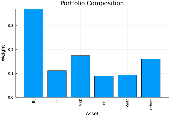
The cumulative returns of the portfolio over the sample.
plot_portfolio_cumulative_returns(res, rd)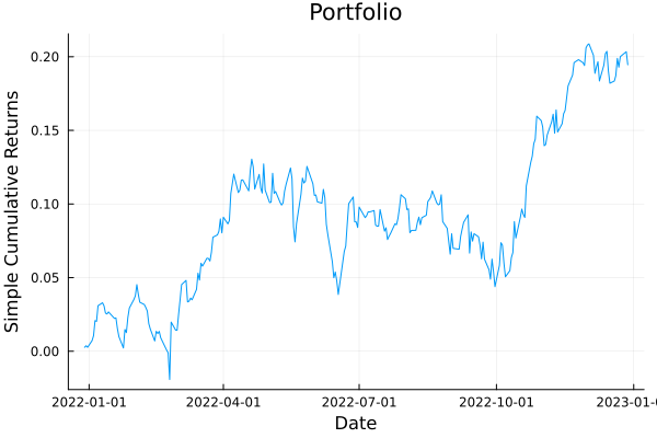
A histogram of the portfolio returns, with markers for the value at risk and the conditional value at risk.
plot_histogram(res, rd)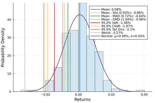
The drawdowns, each the loss from the highest value the portfolio reached before it.
plot_drawdowns(res, rd)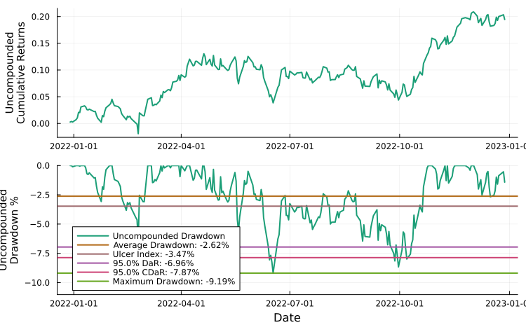
4. Finite allocation
The weights are fractions of capital, but an investor buys whole shares with a fixed amount of cash. A finite allocation turns the weights, the latest prices and the cash into a number of shares per asset. We use DiscreteAllocation, which solves a mixed-integer programme for the best whole-share portfolio. The library also has a greedy method that can allocate fractional shares, and Finite allocation compares the two.
A mixed-integer programme needs a solver that supports it, and we use HiGHS.
using HiGHSmip_slv = Solver(; name = :highs1, solver = HiGHS.Optimizer, settings = Dict("log_to_console" => false), check_sol = (; allow_local = true, allow_almost = true))da = DiscreteAllocation(; slv = mip_slv)DiscreteAllocation
slv ┼ Solver
│ name ┼ Symbol: :highs1
│ solver ┼ DataType: HiGHS.Optimizer
│ settings ┼ Dict{String, Bool}: Dict{String, Bool}("log_to_console" => 0)
│ check_sol ┼ @NamedTuple{allow_local::Bool, allow_almost::Bool}: (allow_local = true, allow_almost = true)
│ add_bridges ┴ Bool: true
sc ┼ Int64: 1
so ┼ Int64: 1
wf ┼ AbsoluteErrorWeightFinaliser()
fb ┼ GreedyAllocation
│ unit ┼ Int64: 1
│ args ┼ Tuple{}: ()
│ kwargs ┼ @NamedTuple{}: NamedTuple()
│ fb ┴ nothing
The allocation needs three inputs. The weights come from the optimisation, the latest prices are the last row of the price table X, and we invest 4206.9 USD.
A FiniteAllocationInput takes the three. It also takes a time horizon and fees, which this page does not use.
mip_res = optimise(da, FiniteAllocationInput(; w = res.w, prices = vec(values(X[end])), cash = 4206.9))DiscreteAllocationResult
retcode ┼ OptimisationSuccess
│ res ┴ nothing
s_retcode ┼ nothing
l_retcode ┼ OptimisationSuccess
│ res ┴ Dict{Any, Any}: Dict{Any, Any}()
shares ┼ 20-element SubArray{Float64, 1, Matrix{Float64}, Tuple{Base.Slice{Base.OneTo{Int64}}, Int64}, true}
cost ┼ 20-element SubArray{Float64, 1, Matrix{Float64}, Tuple{Base.Slice{Base.OneTo{Int64}}, Int64}, true}
w ┼ 20-element SubArray{Float64, 1, Matrix{Float64}, Tuple{Base.Slice{Base.OneTo{Int64}}, Int64}, true}
cash ┼ Float64: 8.471999999997934
fees ┼ Float64: 0.0
s_model ┼ nothing
l_model ┼ A JuMP Model
│ ├ solver: HiGHS
│ ├ objective_sense: MIN_SENSE
│ │ └ objective_function_type: AffExpr
│ ├ num_variables: 21
│ ├ num_constraints: 42
│ │ ├ AffExpr in MOI.GreaterThan{Float64}: 1
│ │ ├ Vector{AffExpr} in MOI.NormOneCone: 1
│ │ ├ VariableRef in MOI.GreaterThan{Float64}: 20
│ │ └ VariableRef in MOI.Integer: 20
│ └ Names registered in the model
│ └ :cabs_err, :cr, :fee, :r, :sc, :so, :u, :x
fb ┴ nothing
This result has different fields from the optimisation result. The discrete allocation solves the long and the short positions apart and then combines them, and the fields that start with l_ or s_ belong to the two halves.
The table below puts the shares, their cost, the optimised weights and the weights of the allocation side by side.
pretty_table(DataFrame(:assets => rd.nx, :shares => mip_res.shares, :cost => mip_res.cost, :opt_weights => res.w, :mip_weights => mip_res.w); formatters = [mipresfmt])┌────────┬─────────┬─────────┬─────────────┬─────────────┐
│ assets │ shares │ cost │ opt_weights │ mip_weights │
│ String │ Float64 │ Float64 │ Float64 │ Float64 │
├────────┼─────────┼─────────┼─────────────┼─────────────┤
│ AAPL │ 0.0 │ 0.0 │ 0.0 % │ 0.0 % │
│ AMD │ 0.0 │ 0.0 │ 0.0 % │ 0.0 % │
│ BAC │ 0.0 │ 0.0 │ 0.0 % │ 0.0 % │
│ BBY │ 0.0 │ 0.0 │ 0.0 % │ 0.0 % │
│ CVX │ 2.0 │ 347.456 │ 7.432 % │ 8.276 % │
│ GE │ 0.0 │ 0.0 │ 0.806 % │ 0.0 % │
│ HD │ 0.0 │ 0.0 │ 0.0 % │ 0.0 % │
│ JNJ │ 9.0 │ 1566.77 │ 36.974 % │ 37.318 % │
│ JPM │ 0.0 │ 0.0 │ 0.749 % │ 0.0 % │
│ KO │ 6.0 │ 375.654 │ 11.161 % │ 8.947 % │
│ LLY │ 0.0 │ 0.0 │ 0.0 % │ 0.0 % │
│ MRK │ 7.0 │ 767.067 │ 17.467 % │ 18.27 % │
│ MSFT │ 0.0 │ 0.0 │ 0.0 % │ 0.0 % │
│ PEP │ 2.0 │ 358.556 │ 8.978 % │ 8.54 % │
│ PFE │ 0.0 │ 0.0 │ 0.0 % │ 0.0 % │
│ PG │ 1.0 │ 149.133 │ 2.353 % │ 3.552 % │
│ RRC │ 0.0 │ 0.0 │ 0.0 % │ 0.0 % │
│ UNH │ 0.0 │ 0.0 │ 0.0 % │ 0.0 % │
│ WMT │ 3.0 │ 420.543 │ 9.355 % │ 10.017 % │
│ XOM │ 2.0 │ 213.254 │ 4.725 % │ 5.079 % │
└────────┴─────────┴─────────┴─────────────┴─────────────┘The weights of the allocation differ from the optimised weights, because a whole number of shares at a fixed cash amount can only come close to them. The cash property of the result is the cash left over. We print it beside the starting cash less the sum of the costs. When the input has fees, the allocation also subtracts the fees from the cash left over.
println("cash left over: $(round(mip_res.cash; digits = 2)), starting cash less the costs: $(round(4206.9 - sum(mip_res.cost); digits = 2))")cash left over: 8.47, starting cash less the costs: 8.47The cost of each asset is its number of shares times its price, and the next cell compares the two.
println("cost of shares ≈ cost of portfolio: $(all(isapprox.(mip_res.shares .* vec(values(X[end])), mip_res.cost)))")cost of shares ≈ cost of portfolio: trueThe last plot puts the optimised weights and the weights of the allocation side by side. The two differ where the allocation rounds a weight to whole shares.
plot_stacked_bar_composition([res, mip_res], rd)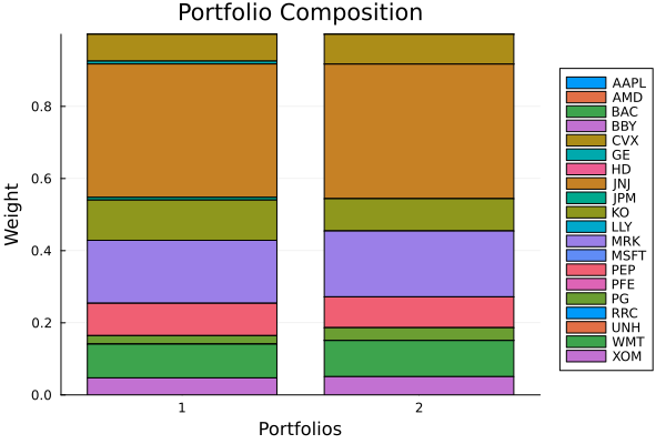
This page was generated using Literate.jl.