factory(a::Union{Nothing, <:AbstractEstimator, <:AbstractAlgorithm,
                 <:AbstractResult}, args...; kwargs...) -> a
factory(a::AbstractVector{<:Union{Nothing, <:AbstractEstimator, <:AbstractAlgorithm,
                                  <:AbstractResult}}, args...; kwargs...) -> Vector
No-op factory function for constructing objects with a uniform interface.
factory(a::Union{Nothing, <:AbstractEstimator, <:AbstractAlgorithm,
                 <:AbstractResult}, args...; kwargs...) -> a
factory(a::AbstractVector{<:Union{Nothing, <:AbstractEstimator, <:AbstractAlgorithm,
                                  <:AbstractResult}}, args...; kwargs...) -> Vector
No-op factory function for constructing objects with a uniform interface.
factory(a::Union{Nothing, <:AbstractEstimator, <:AbstractAlgorithm,
                 <:AbstractResult}, args...; kwargs...) -> a
factory(a::AbstractVector{<:Union{Nothing, <:AbstractEstimator, <:AbstractAlgorithm,
                                  <:AbstractResult}}, args...; kwargs...) -> Vector
No-op factory function for constructing objects with a uniform interface.
factory(a::Union{Nothing, <:AbstractEstimator, <:AbstractAlgorithm,
                 <:AbstractResult}, args...; kwargs...) -> a
factory(a::AbstractVector{<:Union{Nothing, <:AbstractEstimator, <:AbstractAlgorithm,
                                  <:AbstractResult}}, args...; kwargs...) -> Vector
No-op factory function for constructing objects with a uniform interface.
factory(a::Union{Nothing, <:AbstractEstimator, <:AbstractAlgorithm,
                 <:AbstractResult}, args...; kwargs...) -> a
factory(a::AbstractVector{<:Union{Nothing, <:AbstractEstimator, <:AbstractAlgorithm,
                                  <:AbstractResult}}, args...; kwargs...) -> Vector
No-op factory function for constructing objects with a uniform interface.
factory(a::Union{Nothing, <:AbstractEstimator, <:AbstractAlgorithm,
                 <:AbstractResult}, args...; kwargs...) -> a
factory(a::AbstractVector{<:Union{Nothing, <:AbstractEstimator, <:AbstractAlgorithm,
                                  <:AbstractResult}}, args...; kwargs...) -> Vector
No-op factory function for constructing objects with a uniform interface.
prices_to_returns(
    X::TimeSeries.TimeArray,
    F::Option{<:TimeSeries.TimeArray} = nothing;
    B::Option{<:TimeSeries.TimeArray} = nothing,
    iv::Option{<:TimeSeries.TimeArray} = nothing,
    ivpa::Option{<:Num_VecNum} = nothing,
    ret_method::Symbol = :simple, padding::Bool = false,
    missing_col_percent::Number = 1.0,
    missing_row_percent::Option{<:Number} = 1.0,
    collapse_args::Tuple = (),
    map_func::Option{<:Function} = nothing,
    join_method::Symbol = :outer,
    impute_method = nothing,
    nz::Option{<:VecStr} = nothing,
    Z::Option{<:MatNum_Arr3Num} = nothing
) -> ReturnsResult
Convert TimeSeries.TimeArray price data to returns.
factory(a::Union{Nothing, <:AbstractEstimator, <:AbstractAlgorithm,
                 <:AbstractResult}, args...; kwargs...) -> a
factory(a::AbstractVector{<:Union{Nothing, <:AbstractEstimator, <:AbstractAlgorithm,
                                  <:AbstractResult}}, args...; kwargs...) -> Vector
No-op factory function for constructing objects with a uniform interface.
factory(a::Union{Nothing, <:AbstractEstimator, <:AbstractAlgorithm,
                 <:AbstractResult}, args...; kwargs...) -> a
factory(a::AbstractVector{<:Union{Nothing, <:AbstractEstimator, <:AbstractAlgorithm,
                                  <:AbstractResult}}, args...; kwargs...) -> Vector
No-op factory function for constructing objects with a uniform interface.
factory(
    ce::StatsBase.CovarianceEstimator,
    args...;
    kwargs...
) -> StatsBase.CovarianceEstimator
Fallback for covariance estimator factory methods.
factory(a::Union{Nothing, <:AbstractEstimator, <:AbstractAlgorithm,
                 <:AbstractResult}, args...; kwargs...) -> a
factory(a::AbstractVector{<:Union{Nothing, <:AbstractEstimator, <:AbstractAlgorithm,
                                  <:AbstractResult}}, args...; kwargs...) -> Vector
No-op factory function for constructing objects with a uniform interface.
factory(re::GeneralisedLinearModel, w::ObsWeights) -> GeneralisedLinearModelReturn a new GeneralisedLinearModel regression target with observation weights w added to the keyword arguments.
factory(re::LinearModel, w::ObsWeights) -> LinearModelReturn a new LinearModel regression target with observation weights w added to the keyword arguments.
factory(drtgt::DimensionReductionTarget, args...; kwargs...) -> DimensionReductionTargetNo-op factory for DimensionReductionTarget subtypes.
factory(a::Union{Nothing, <:AbstractEstimator, <:AbstractAlgorithm,
                 <:AbstractResult}, args...; kwargs...) -> a
factory(a::AbstractVector{<:Union{Nothing, <:AbstractEstimator, <:AbstractAlgorithm,
                                  <:AbstractResult}}, args...; kwargs...) -> Vector
No-op factory function for constructing objects with a uniform interface.
factory(a::Union{Nothing, <:AbstractEstimator, <:AbstractAlgorithm,
                 <:AbstractResult}, args...; kwargs...) -> a
factory(a::AbstractVector{<:Union{Nothing, <:AbstractEstimator, <:AbstractAlgorithm,
                                  <:AbstractResult}}, args...; kwargs...) -> Vector
No-op factory function for constructing objects with a uniform interface.
struct Solver{__T_name, __T_solver, __T_settings, __T_check_sol, __T_add_bridges} <: AbstractEstimatorConfigures one solver backend, its attributes, and the statuses its solutions must reach.
factory(
    alg::AbstractPhylogenyAlgorithm,
    args...;
    kwargs...
) -> AbstractClustersAlgorithm
Return the phylogeny algorithm alg unchanged.
factory(
    pl::Union{AbstractPhylogenyEstimator, AbstractPhylogenyResult},
    args...;
    kwargs...
) -> NetworkEstimator{<:CovarianceEstimator, <:AbstractDistanceEstimator, KruskalTree{Tuple{}, @NamedTuple{}}, <:AbstractSeparationAlgorithm}
Return the phylogeny estimator or result pl unchanged.
factory(
    alg::AbstractClustersAlgorithm,
    args...;
    kwargs...
) -> AbstractClustersAlgorithm
Return the clustering algorithm alg unchanged.
prior(pr::AbstractPriorEstimator, rd::ReturnsResult; kwargs...)Compute prior information from asset and/or factor returns using a prior estimator.
prior(pr::AbstractPriorResult, args...; kwargs...)Propagate or pass through prior result objects.
struct EmpiricalPrior{__T_ce, __T_me, __T_horizon} <: AbstractLowOrderPriorEstimator_AEmpirical prior estimator for asset returns.
prior(pe::EmpiricalPrior{<:Any, <:Any, <:Number}, X::MatNum, args...; dims::Int = 1,
      kwargs...)
Compute empirical prior moments for asset returns with investment horizon adjustment.
prior(pe::EmpiricalPrior{<:Any, <:Any, Nothing}, X::MatNum, args...; dims::Int = 1,
      kwargs...)
Compute empirical prior moments for asset returns (no horizon adjustment).
prior(pe::HighOrderPriorEstimator, X::MatNum, F::Option{<:MatNum} = nothing; dims::Int = 1, kwargs...)Compute high order prior moments for asset returns using a composite estimator.
prior(pe::BlackLittermanPrior, X::MatNum, F::Option{<:MatNum} = nothing;
      dims::Int = 1, strict::Bool = false, kwargs...)
Compute the Black-Litterman prior moments for asset returns.
prior(pe::MeucciEntropyPoolingPrior, X::MatNum, F::Option{<:MatNum} = nothing;
      dims::Int = 1, strict::Bool = false, kwargs...)
Compute entropy pooling prior moments for asset returns.
prior(pe::EntropyPoolingPrior, X::MatNum, F::Option{<:MatNum} = nothing;
      dims::Int = 1, strict::Bool = false, kwargs...)
Compute the entropy pooling prior of asset returns with tail views.
prior(pe::OpinionPoolingPrior, X::MatNum, F::Option{<:MatNum} = nothing;
      dims::Int = 1, strict::Bool = false, kwargs...)
Compute opinion pooling prior moments for asset returns.
prior(pe::FeaturePrior, X::MatNum, F::Option{<:MatNum} = nothing;
      dims::Int = 1, kwargs...)
Compute the wrapped prior's moments and attach a feature matrix to them.
factory(tn::VecTnE_Tn, w::VecNum)Create new turnover constraints or estimators with updated portfolio weights.
factory(tn::Turnover, w::VecNum)Create a new Turnover constraint with updated portfolio weights.
factory(tn::TurnoverEstimator, w::VecNum)Create a new TurnoverEstimator with updated portfolio weights.
factory(tr::WeightsTracking, w::VecNum)Construct a new WeightsTracking object with updated portfolio weights.
struct Frontier{__T_N, __T_factor, __T_bound} <: AbstractAlgorithmSweeps the efficient frontier by solving the model once at each of N evenly spaced bound values.
factory(
    rs::AbstractBaseRiskMeasure,
    args...;
    kwargs...
) -> GenericValueatRiskRange{RiskMeasureSettings{__T_scale, __T_ub, __T_rke}} where {__T_scale, __T_ub, __T_rke}
Return the risk measure rs unchanged.
struct Variance{__T_settings, __T_sigma, __T_chol, __T_rc, __T_alg} <: RiskMeasureRepresents the portfolio variance using a covariance matrix.
factory(r::UncertaintySetVariance, pr::AbstractPriorResult, ::Any,
        ucs::Option{<:UcSE_UcS} = nothing, args...;
        kwargs...)
Create an instance of UncertaintySetVariance by selecting the uncertainty set and covariance matrix from the risk-measure instance or falling back to the prior result.
factory(
    r::StandardDeviation,
    pr::AbstractPriorResult,
    args...;
    kwargs...
) -> Union{StandardDeviation{__T_settings, __T_sigma, Nothing} where {__T_settings, __T_sigma}, StandardDeviation{RiskMeasureSettings{__T_scale, __T_ub, __T_rke}, var"#s179", <:AbstractMatrix{var"#s90"}} where {__T_scale, __T_ub, __T_rke, var"#s90"<:(Union{var"#s89", var"#s88"} where {var"#s89"<:Number, var"#s88"<:AbstractJuMPScalar}), var"#s179"<:AbstractMatrix{var"#s90"}, var"#s90"<:(Union{var"#s89", var"#s88"} where {var"#s89"<:Number, var"#s88"<:AbstractJuMPScalar})}}
Create an instance of StandardDeviation by resolving a Deferred Quantity in sigma, then falling back to the prior result for the covariance matrix and its factorisation as a pair.
factory(
    r::Variance,
    pr::AbstractPriorResult,
    args...;
    kwargs...
) -> Variance{RiskMeasureSettings{__T_scale, __T_ub, __T_rke}, _A, _B, _C, <:VarianceFormulation} where {__T_scale, __T_ub, __T_rke, _A, _B, _C}
Create an instance of Variance by resolving a Deferred Quantity in sigma, then falling back to the prior result for the covariance matrix and its factorisation.
factory(
    r::HighOrderMoment,
    pr::AbstractPriorResult,
    args...;
    kwargs...
) -> HighOrderMoment{RiskMeasureSettings{__T_scale, __T_ub, __T_rke}, _A, _B, <:HighOrderMomentMeasureAlgorithm} where {__T_scale, __T_ub, __T_rke, _A, _B}
Create an instance of HighOrderMoment by selecting observation weights, expected returns, and algorithm from the risk-measure instance or falling back to the prior result.
factory(
    r::LowOrderMoment,
    pr::AbstractPriorResult,
    args...;
    kwargs...
) -> LowOrderMoment{RiskMeasureSettings{__T_scale, __T_ub, __T_rke}, _A, _B, <:LowOrderMomentMeasureAlgorithm} where {__T_scale, __T_ub, __T_rke, _A, _B}
Create an instance of LowOrderMoment by selecting observation weights, expected returns, and algorithm from the risk-measure instance or falling back to the prior result.
factory(
    alg::MomentMeasureAlgorithm,
    args...;
    kwargs...
) -> StandardisedHighOrderMoment{<:AbstractVarianceEstimator, <:UnstandardisedHighOrderMomentMeasureAlgorithm}
Return the moment measure algorithm alg unchanged.
factory(
    alg::StandardisedHighOrderMoment,
    w::Union{DynamicAbstractWeights, AbstractWeights}
) -> StandardisedHighOrderMoment{<:AbstractVarianceEstimator, <:UnstandardisedHighOrderMomentMeasureAlgorithm}
Return a new StandardisedHighOrderMoment with observation weights w applied to the underlying variance estimator.
factory(
    r::Kurtosis,
    pr::HighOrderPrior,
    args...;
    kwargs...
) -> Kurtosis{RiskMeasureSettings{__T_scale, __T_ub, __T_rke}, _A, _B, _C, _D, <:AbstractMomentAlgorithm, <:SecondMomentFormulation, Nothing} where {__T_scale, __T_ub, __T_rke, _A, _B, _C, _D}
Create an instance of Kurtosis by selecting the cokurtosis matrix, expected returns, and weights from the risk-measure instance or falling back to a HighOrderPrior result.
factory(
    r::Kurtosis,
    pr::LowOrderPrior,
    args...;
    kwargs...
) -> Kurtosis{RiskMeasureSettings{__T_scale, __T_ub, __T_rke}, _A, _B, _C, _D, <:AbstractMomentAlgorithm, <:SecondMomentFormulation, Nothing} where {__T_scale, __T_ub, __T_rke, _A, _B, _C, _D}
Create an instance of Kurtosis from a LowOrderPrior result (cokurtosis matrix is not used).
factory(
    r::NegativeSkewness,
    pr::HighOrderPrior,
    args...;
    kwargs...
) -> NegativeSkewness{RiskMeasureSettings{__T_scale, __T_ub, __T_rke}, <:AbstractMatrixProcessingEstimator} where {__T_scale, __T_ub, __T_rke}
Create an instance of NegativeSkewness by resolving a Deferred Quantity in sk, then falling back to a HighOrderPrior result for the coskewness matrix and its spectral decomposition.
factory(
    r::NegativeSkewness,
    pr::LowOrderPrior,
    args...;
    kwargs...
) -> NegativeSkewness
Resolve a Deferred Quantity in NegativeSkewness's sk slot against a LowOrderPrior result, and otherwise return r unchanged.
factory(
    alg::DistributionValueatRisk,
    pr::AbstractPriorResult,
    args...;
    kwargs...
) -> DistributionValueatRisk{_A, _B, _C, Nothing, <:Distributions.Distribution{F, S}} where {_A, _B, _C, F<:Distributions.VariateForm, S<:Distributions.ValueSupport}
Create an instance of DistributionValueatRisk by resolving its Deferred Quantities, then falling back to the prior result for whatever is still unstated.
factory(
    alg::ValueatRiskFormulation,
    args...;
    kwargs...
) -> DistributionValueatRisk{_A, _B, _C, Nothing, <:Distributions.Distribution{F, S}} where {_A, _B, _C, F<:Distributions.VariateForm, S<:Distributions.ValueSupport}
Return the Value-at-Risk formulation alg unchanged.
factory(
    r::TurnoverRiskMeasure,
    ,
    ,
    ;
    ...
) -> TurnoverRiskMeasure
factory(
    r::TurnoverRiskMeasure,
    ,
    ,
    ,
    w::Union{Nothing, AbstractVector{<:Union{var"#s89", var"#s88"} where {var"#s89"<:Number, var"#s88"<:AbstractJuMPScalar}}},
    args...;
    kwargs...
) -> TurnoverRiskMeasure
Create an instance of TurnoverRiskMeasure from a full optimisation context, forwarding the optional weight argument w to factory(r, w).
factory(
    r::TurnoverRiskMeasure,
    w::AbstractVector{<:Union{var"#s89", var"#s88"} where {var"#s89"<:Number, var"#s88"<:AbstractJuMPScalar}}
) -> TurnoverRiskMeasure
Create an instance of TurnoverRiskMeasure updating the reference weights to w.
factory(
    tr::RiskTrackingError,
    pr::AbstractPriorResult,
    slv,
    ucs;
    ...
) -> RiskTrackingError{WeightsTracking{__T_fees, __T_w, __T_fixed}, _A, <:Number, <:VariableTracking} where {__T_fees, __T_w, __T_fixed, _A}
factory(
    tr::RiskTrackingError,
    pr::AbstractPriorResult,
    slv,
    ucs,
    w::Union{Nothing, AbstractVector{<:Union{var"#s89", var"#s88"} where {var"#s89"<:Number, var"#s88"<:AbstractJuMPScalar}}},
    args...;
    kwargs...
) -> RiskTrackingError{WeightsTracking{__T_fees, __T_w, __T_fixed}, _A, <:Number, <:VariableTracking} where {__T_fees, __T_w, __T_fixed, _A}
Create an instance of RiskTrackingError updating the inner benchmark and risk measure from the prior result and solver context.
factory(
    tr::RiskTrackingError,
    w::AbstractVector{<:Union{var"#s89", var"#s88"} where {var"#s89"<:Number, var"#s88"<:AbstractJuMPScalar}}
) -> RiskTrackingError{WeightsTracking{__T_fees, __T_w, __T_fixed}, _A, <:Number, <:VariableTracking} where {__T_fees, __T_w, __T_fixed, _A}
Create an instance of RiskTrackingError updating the inner benchmark and risk measure from new portfolio weights w.
factory(
    r::RiskTrackingRiskMeasure,
    pr::AbstractPriorResult,
    args...;
    kwargs...
) -> RiskTrackingRiskMeasure{RiskMeasureSettings{__T_scale, __T_ub, __T_rke}, WeightsTracking{__T_fees, __T_w, __T_fixed}, _A, <:VariableTracking} where {__T_scale, __T_ub, __T_rke, __T_fees, __T_w, __T_fixed, _A}
Create an instance of RiskTrackingRiskMeasure updating the inner risk measure from the prior result.
factory(
    r::RiskTrackingRiskMeasure,
    w::AbstractVector{<:Union{var"#s89", var"#s88"} where {var"#s89"<:Number, var"#s88"<:AbstractJuMPScalar}}
) -> RiskTrackingRiskMeasure{RiskMeasureSettings{__T_scale, __T_ub, __T_rke}, WeightsTracking{__T_fees, __T_w, __T_fixed}, _A, <:VariableTracking} where {__T_scale, __T_ub, __T_rke, __T_fees, __T_w, __T_fixed, _A}
Create an instance of RiskTrackingRiskMeasure updating the inner benchmark and risk measure from new portfolio weights w.
factory(
    r::TrackingRiskMeasure,
    w::AbstractVector{<:Union{var"#s89", var"#s88"} where {var"#s89"<:Number, var"#s88"<:AbstractJuMPScalar}}
) -> TrackingRiskMeasure{RiskMeasureSettings{__T_scale, __T_ub, __T_rke}, <:AbstractTrackingAlgorithm, <:NormError} where {__T_scale, __T_ub, __T_rke}
Create an instance of TrackingRiskMeasure updating the inner tracking specification with new weights w.
factory(
    r::TrackingRiskMeasure,
    ,
    ,
    ,
    w::AbstractVector{<:Union{var"#s89", var"#s88"} where {var"#s89"<:Number, var"#s88"<:AbstractJuMPScalar}},
    args...;
    kwargs...
) -> TrackingRiskMeasure{RiskMeasureSettings{__T_scale, __T_ub, __T_rke}, <:AbstractTrackingAlgorithm, <:NormError} where {__T_scale, __T_ub, __T_rke}
Create an instance of TrackingRiskMeasure from a full optimisation context, forwarding w to factory(r, w).
factory(
    r::Skewness,
    pr::HighOrderPrior,
    args...;
    kwargs...
) -> Skewness{MaxRiskMeasureSettings{Float64, Nothing, Bool}, var"#s179", _A, _B, _C, Nothing} where {var"#s179"<:AbstractVarianceEstimator, _A, _B, _C}
Create an instance of Skewness by selecting observation weights and expected returns from the risk-measure instance or falling back to the prior result.
factory(
    r::Skewness,
    pr::LowOrderPrior,
    args...;
    kwargs...
) -> Skewness{MaxRiskMeasureSettings{Float64, Nothing, Bool}, var"#s179", _A, _B, _C, Nothing} where {var"#s179"<:AbstractVarianceEstimator, _A, _B, _C}
Create an instance of Skewness from a LowOrderPrior result, selecting observation weights and expected returns while preserving the coskewness matrix from the risk measure.
factory(
    r::VarianceSkewKurtosis,
    pr::AbstractPriorResult,
    args...;
    kwargs...
) -> VarianceSkewKurtosis{RiskMeasureSettings{__T_scale, __T_ub, __T_rke}, _A, Skewness{__T_settings, __T_ve, __T_sk, __T_w, __T_mu, __T_pe}, _B, Nothing} where {__T_scale, __T_ub, __T_rke, _A, __T_settings, __T_ve, __T_sk, __T_w, __T_mu, __T_pe, _B}
Create an instance of VarianceSkewKurtosis by fanning pe out over its three children, then threading pr into each of them.
factory(a::Union{Nothing, <:AbstractEstimator, <:AbstractAlgorithm,
                 <:AbstractResult}, args...; kwargs...) -> a
factory(a::AbstractVector{<:Union{Nothing, <:AbstractEstimator, <:AbstractAlgorithm,
                                  <:AbstractResult}}, args...; kwargs...) -> Vector
factory(
    rs::AbstractBaseRiskMeasure,
    args...;
    kwargs...
) -> GenericValueatRiskRange{RiskMeasureSettings{__T_scale, __T_ub, __T_rke}} where {__T_scale, __T_ub, __T_rke}
No-op factory function for constructing objects with a uniform interface.
factory(a::Union{Nothing, <:AbstractEstimator, <:AbstractAlgorithm,
                 <:AbstractResult}, args...; kwargs...) -> a
factory(a::AbstractVector{<:Union{Nothing, <:AbstractEstimator, <:AbstractAlgorithm,
                                  <:AbstractResult}}, args...; kwargs...) -> Vector
factory(
    rs::AbstractBaseRiskMeasure,
    args...;
    kwargs...
) -> GenericValueatRiskRange{RiskMeasureSettings{__T_scale, __T_ub, __T_rke}} where {__T_scale, __T_ub, __T_rke}
No-op factory function for constructing objects with a uniform interface.
factory(a::Union{Nothing, <:AbstractEstimator, <:AbstractAlgorithm,
                 <:AbstractResult}, args...; kwargs...) -> a
factory(a::AbstractVector{<:Union{Nothing, <:AbstractEstimator, <:AbstractAlgorithm,
                                  <:AbstractResult}}, args...; kwargs...) -> Vector
factory(
    rs::AbstractBaseRiskMeasure,
    args...;
    kwargs...
) -> GenericValueatRiskRange{RiskMeasureSettings{__T_scale, __T_ub, __T_rke}} where {__T_scale, __T_ub, __T_rke}
No-op factory function for constructing objects with a uniform interface.
factory(a::Union{Nothing, <:AbstractEstimator, <:AbstractAlgorithm,
                 <:AbstractResult}, args...; kwargs...) -> a
factory(a::AbstractVector{<:Union{Nothing, <:AbstractEstimator, <:AbstractAlgorithm,
                                  <:AbstractResult}}, args...; kwargs...) -> Vector
factory(
    rs::AbstractBaseRiskMeasure,
    args...;
    kwargs...
) -> GenericValueatRiskRange{RiskMeasureSettings{__T_scale, __T_ub, __T_rke}} where {__T_scale, __T_ub, __T_rke}
No-op factory function for constructing objects with a uniform interface.
factory(a::Union{Nothing, <:AbstractEstimator, <:AbstractAlgorithm,
                 <:AbstractResult}, args...; kwargs...) -> a
factory(a::AbstractVector{<:Union{Nothing, <:AbstractEstimator, <:AbstractAlgorithm,
                                  <:AbstractResult}}, args...; kwargs...) -> Vector
factory(
    rs::AbstractBaseRiskMeasure,
    args...;
    kwargs...
) -> GenericValueatRiskRange{RiskMeasureSettings{__T_scale, __T_ub, __T_rke}} where {__T_scale, __T_ub, __T_rke}
No-op factory function for constructing objects with a uniform interface.
factory(res::NonFiniteAllocationOptimisationResult, fb::Option{<:OptE_Opt})Rebuild a continuous optimisation result with an updated fallback optimiser fb.
factory(td::TimeDependent, args...) -> TimeDependentApply factory through a TimeDependent schedule: to each vector entry and to the default, rebuilding the schedule.
factory(
    opt::Union{NonFiniteAllocationOptimisationEstimator, NonFiniteAllocationOptimisationResult},
    _
) -> FactorRiskContribution{JuMPOptimiser{__T_pe, __T_slv, __T_wb, __T_bgt, __T_sbgt, __T_gbgt, __T_xbgt, __T_lt, __T_st, __T_lcse, __T_cte, __T_gcarde, __T_sgcarde, __T_smtx, __T_sgmtx, __T_slt, __T_sst, __T_sglt, __T_sgst, __T_tn, __T_fees, __T_sets, __T_tr, __T_ple, __T_ret, __T_sca, __T_ccnt, __T_cobj, __T_sc, __T_so, __T_ss, __T_card, __T_scard, __T_l2c, __T_lpc, __T_linfc, __T_l1, __T_l2, __T_linf, __T_lp, __T_brt, __T_x_src, __T_z_src, __T_strict}, _A, _B, _C, _D, _E, _F, Bool} where {__T_pe, __T_slv, __T_wb, __T_bgt, __T_sbgt, __T_gbgt, __T_xbgt, __T_lt, __T_st, __T_lcse, __T_cte, __T_gcarde, __T_sgcarde, __T_smtx, __T_sgmtx, __T_slt, __T_sst, __T_sglt, __T_sgst, __T_tn, __T_fees, __T_sets, __T_tr, __T_ple, __T_ret, __T_sca, __T_ccnt, __T_cobj, __T_sc, __T_so, __T_ss, __T_card, __T_scard, __T_l2c, __T_lpc, __T_linfc, __T_l1, __T_l2, __T_linf, __T_lp, __T_brt, __T_x_src, __T_z_src, __T_strict, _A, _B, _C, _D, _E, _F}
Return opt unchanged.
optimise(
    opt::OptimisationEstimator,
    args...;
    kwargs...
) -> Union{HierarchicalRiskParityResult{HierarchicalResult{__T_pr, __T_clr, __T_wb, __T_fees, __T_retcode, __T_w}, <:AbstractBaseRiskMeasure, <:Scalariser, Nothing} where {__T_pr, __T_clr, __T_wb, __T_fees, __T_retcode, __T_w}, HierarchicalRiskParityResult{HierarchicalResult{__T_pr, __T_clr, __T_wb, __T_fees, __T_retcode, __T_w}, <:AbstractVector{var"#s936"}, <:Scalariser, Nothing} where {__T_pr, __T_clr, __T_wb, __T_fees, __T_retcode, __T_w, var"#s936"<:AbstractBaseRiskMeasure}}
High level optimisation function that wraps around estimator-specific optimisation functions.
optimise(opt::OptimisationEstimator, args...; kwargs...) -> OptimisationResult
optimise(opt::OptimisationResult, args...; kwargs...) -> OptimisationResult
Run portfolio optimisation using the given estimator opt and return an OptimisationResult.
optimise(
    td::Union{TimeDependent{<:AbstractVector{<:Union{var"#s936", var"#s935"} where {var"#s936"<:NonFiniteAllocationOptimisationEstimator, var"#s935"<:NonFiniteAllocationOptimisationResult}}}, TimeDependent{<:TimeDependentOptimiserCallable}, TimeDependent{<:PreviousWeightsFunction}, TimeDependent{<:Union{Function, Type}}},
    args...;
    kwargs...
) -> Any
Optimise with a TimeDependent schedule standing in for the optimiser, outside any fold loop.
factory(a::Union{Nothing, <:AbstractEstimator, <:AbstractAlgorithm,
                 <:AbstractResult}, args...; kwargs...) -> a
factory(a::AbstractVector{<:Union{Nothing, <:AbstractEstimator, <:AbstractAlgorithm,
                                  <:AbstractResult}}, args...; kwargs...) -> Vector
factory(res::NonFiniteAllocationOptimisationResult, fb::Option{<:OptE_Opt})
factory(
    opt::Union{NonFiniteAllocationOptimisationEstimator, NonFiniteAllocationOptimisationResult},
    _
) -> FactorRiskContribution{JuMPOptimiser{__T_pe, __T_slv, __T_wb, __T_bgt, __T_sbgt, __T_gbgt, __T_xbgt, __T_lt, __T_st, __T_lcse, __T_cte, __T_gcarde, __T_sgcarde, __T_smtx, __T_sgmtx, __T_slt, __T_sst, __T_sglt, __T_sgst, __T_tn, __T_fees, __T_sets, __T_tr, __T_ple, __T_ret, __T_sca, __T_ccnt, __T_cobj, __T_sc, __T_so, __T_ss, __T_card, __T_scard, __T_l2c, __T_lpc, __T_linfc, __T_l1, __T_l2, __T_linf, __T_lp, __T_brt, __T_x_src, __T_z_src, __T_strict}, _A, _B, _C, _D, _E, _F, Bool} where {__T_pe, __T_slv, __T_wb, __T_bgt, __T_sbgt, __T_gbgt, __T_xbgt, __T_lt, __T_st, __T_lcse, __T_cte, __T_gcarde, __T_sgcarde, __T_smtx, __T_sgmtx, __T_slt, __T_sst, __T_sglt, __T_sgst, __T_tn, __T_fees, __T_sets, __T_tr, __T_ple, __T_ret, __T_sca, __T_ccnt, __T_cobj, __T_sc, __T_so, __T_ss, __T_card, __T_scard, __T_l2c, __T_lpc, __T_linfc, __T_l1, __T_l2, __T_linf, __T_lp, __T_brt, __T_x_src, __T_z_src, __T_strict, _A, _B, _C, _D, _E, _F}
No-op factory function for constructing objects with a uniform interface.
optimise(iv::InverseVolatility{<:Any, <:Any, <:Any, <:Any, Nothing},
         rd::ReturnsResult = ReturnsResult(); dims::Int = 1, kwargs...) -> NaiveOptimisationResult
Run the inverse volatility portfolio optimisation.
factory(a::Union{Nothing, <:AbstractEstimator, <:AbstractAlgorithm,
                 <:AbstractResult}, args...; kwargs...) -> a
factory(a::AbstractVector{<:Union{Nothing, <:AbstractEstimator, <:AbstractAlgorithm,
                                  <:AbstractResult}}, args...; kwargs...) -> Vector
factory(res::NonFiniteAllocationOptimisationResult, fb::Option{<:OptE_Opt})
factory(
    opt::Union{NonFiniteAllocationOptimisationEstimator, NonFiniteAllocationOptimisationResult},
    _
) -> FactorRiskContribution{JuMPOptimiser{__T_pe, __T_slv, __T_wb, __T_bgt, __T_sbgt, __T_gbgt, __T_xbgt, __T_lt, __T_st, __T_lcse, __T_cte, __T_gcarde, __T_sgcarde, __T_smtx, __T_sgmtx, __T_slt, __T_sst, __T_sglt, __T_sgst, __T_tn, __T_fees, __T_sets, __T_tr, __T_ple, __T_ret, __T_sca, __T_ccnt, __T_cobj, __T_sc, __T_so, __T_ss, __T_card, __T_scard, __T_l2c, __T_lpc, __T_linfc, __T_l1, __T_l2, __T_linf, __T_lp, __T_brt, __T_x_src, __T_z_src, __T_strict}, _A, _B, _C, _D, _E, _F, Bool} where {__T_pe, __T_slv, __T_wb, __T_bgt, __T_sbgt, __T_gbgt, __T_xbgt, __T_lt, __T_st, __T_lcse, __T_cte, __T_gcarde, __T_sgcarde, __T_smtx, __T_sgmtx, __T_slt, __T_sst, __T_sglt, __T_sgst, __T_tn, __T_fees, __T_sets, __T_tr, __T_ple, __T_ret, __T_sca, __T_ccnt, __T_cobj, __T_sc, __T_so, __T_ss, __T_card, __T_scard, __T_l2c, __T_lpc, __T_linfc, __T_l1, __T_l2, __T_linf, __T_lp, __T_brt, __T_x_src, __T_z_src, __T_strict, _A, _B, _C, _D, _E, _F}
No-op factory function for constructing objects with a uniform interface.
factory(a::Union{Nothing, <:AbstractEstimator, <:AbstractAlgorithm,
                 <:AbstractResult}, args...; kwargs...) -> a
factory(a::AbstractVector{<:Union{Nothing, <:AbstractEstimator, <:AbstractAlgorithm,
                                  <:AbstractResult}}, args...; kwargs...) -> Vector
factory(res::NonFiniteAllocationOptimisationResult, fb::Option{<:OptE_Opt})
factory(
    opt::Union{NonFiniteAllocationOptimisationEstimator, NonFiniteAllocationOptimisationResult},
    _
) -> FactorRiskContribution{JuMPOptimiser{__T_pe, __T_slv, __T_wb, __T_bgt, __T_sbgt, __T_gbgt, __T_xbgt, __T_lt, __T_st, __T_lcse, __T_cte, __T_gcarde, __T_sgcarde, __T_smtx, __T_sgmtx, __T_slt, __T_sst, __T_sglt, __T_sgst, __T_tn, __T_fees, __T_sets, __T_tr, __T_ple, __T_ret, __T_sca, __T_ccnt, __T_cobj, __T_sc, __T_so, __T_ss, __T_card, __T_scard, __T_l2c, __T_lpc, __T_linfc, __T_l1, __T_l2, __T_linf, __T_lp, __T_brt, __T_x_src, __T_z_src, __T_strict}, _A, _B, _C, _D, _E, _F, Bool} where {__T_pe, __T_slv, __T_wb, __T_bgt, __T_sbgt, __T_gbgt, __T_xbgt, __T_lt, __T_st, __T_lcse, __T_cte, __T_gcarde, __T_sgcarde, __T_smtx, __T_sgmtx, __T_slt, __T_sst, __T_sglt, __T_sgst, __T_tn, __T_fees, __T_sets, __T_tr, __T_ple, __T_ret, __T_sca, __T_ccnt, __T_cobj, __T_sc, __T_so, __T_ss, __T_card, __T_scard, __T_l2c, __T_lpc, __T_linfc, __T_l1, __T_l2, __T_linf, __T_lp, __T_brt, __T_x_src, __T_z_src, __T_strict, _A, _B, _C, _D, _E, _F}
No-op factory function for constructing objects with a uniform interface.
optimise(hrp::HierarchicalRiskParity{<:Any, <:Any, <:Any, <:Nothing},
         rd::ReturnsResult = ReturnsResult(); dims::Int = 1, kwargs...) -> HierarchicalRiskParityResult
Run the Hierarchical Risk Parity portfolio optimisation.
factory(a::Union{Nothing, <:AbstractEstimator, <:AbstractAlgorithm,
                 <:AbstractResult}, args...; kwargs...) -> a
factory(a::AbstractVector{<:Union{Nothing, <:AbstractEstimator, <:AbstractAlgorithm,
                                  <:AbstractResult}}, args...; kwargs...) -> Vector
factory(res::NonFiniteAllocationOptimisationResult, fb::Option{<:OptE_Opt})
factory(
    opt::Union{NonFiniteAllocationOptimisationEstimator, NonFiniteAllocationOptimisationResult},
    _
) -> FactorRiskContribution{JuMPOptimiser{__T_pe, __T_slv, __T_wb, __T_bgt, __T_sbgt, __T_gbgt, __T_xbgt, __T_lt, __T_st, __T_lcse, __T_cte, __T_gcarde, __T_sgcarde, __T_smtx, __T_sgmtx, __T_slt, __T_sst, __T_sglt, __T_sgst, __T_tn, __T_fees, __T_sets, __T_tr, __T_ple, __T_ret, __T_sca, __T_ccnt, __T_cobj, __T_sc, __T_so, __T_ss, __T_card, __T_scard, __T_l2c, __T_lpc, __T_linfc, __T_l1, __T_l2, __T_linf, __T_lp, __T_brt, __T_x_src, __T_z_src, __T_strict}, _A, _B, _C, _D, _E, _F, Bool} where {__T_pe, __T_slv, __T_wb, __T_bgt, __T_sbgt, __T_gbgt, __T_xbgt, __T_lt, __T_st, __T_lcse, __T_cte, __T_gcarde, __T_sgcarde, __T_smtx, __T_sgmtx, __T_slt, __T_sst, __T_sglt, __T_sgst, __T_tn, __T_fees, __T_sets, __T_tr, __T_ple, __T_ret, __T_sca, __T_ccnt, __T_cobj, __T_sc, __T_so, __T_ss, __T_card, __T_scard, __T_l2c, __T_lpc, __T_linfc, __T_l1, __T_l2, __T_linf, __T_lp, __T_brt, __T_x_src, __T_z_src, __T_strict, _A, _B, _C, _D, _E, _F}
No-op factory function for constructing objects with a uniform interface.
optimise(sh::SchurComplementHierarchicalRiskParity{<:Any, <:Any, Nothing},
         rd::ReturnsResult = ReturnsResult(); dims::Int = 1, kwargs...) -> SchurComplementHierarchicalRiskParityResult
Run the Schur Complement Hierarchical Risk Parity portfolio optimisation.
factory(a::Union{Nothing, <:AbstractEstimator, <:AbstractAlgorithm,
                 <:AbstractResult}, args...; kwargs...) -> a
factory(a::AbstractVector{<:Union{Nothing, <:AbstractEstimator, <:AbstractAlgorithm,
                                  <:AbstractResult}}, args...; kwargs...) -> Vector
factory(
    opt::Union{NonFiniteAllocationOptimisationEstimator, NonFiniteAllocationOptimisationResult},
    _
) -> FactorRiskContribution{JuMPOptimiser{__T_pe, __T_slv, __T_wb, __T_bgt, __T_sbgt, __T_gbgt, __T_xbgt, __T_lt, __T_st, __T_lcse, __T_cte, __T_gcarde, __T_sgcarde, __T_smtx, __T_sgmtx, __T_slt, __T_sst, __T_sglt, __T_sgst, __T_tn, __T_fees, __T_sets, __T_tr, __T_ple, __T_ret, __T_sca, __T_ccnt, __T_cobj, __T_sc, __T_so, __T_ss, __T_card, __T_scard, __T_l2c, __T_lpc, __T_linfc, __T_l1, __T_l2, __T_linf, __T_lp, __T_brt, __T_x_src, __T_z_src, __T_strict}, _A, _B, _C, _D, _E, _F, Bool} where {__T_pe, __T_slv, __T_wb, __T_bgt, __T_sbgt, __T_gbgt, __T_xbgt, __T_lt, __T_st, __T_lcse, __T_cte, __T_gcarde, __T_sgcarde, __T_smtx, __T_sgmtx, __T_slt, __T_sst, __T_sglt, __T_sgst, __T_tn, __T_fees, __T_sets, __T_tr, __T_ple, __T_ret, __T_sca, __T_ccnt, __T_cobj, __T_sc, __T_so, __T_ss, __T_card, __T_scard, __T_l2c, __T_lpc, __T_linfc, __T_l1, __T_l2, __T_linf, __T_lp, __T_brt, __T_x_src, __T_z_src, __T_strict, _A, _B, _C, _D, _E, _F}
No-op factory function for constructing objects with a uniform interface.
optimise(hec::HierarchicalEqualRiskContribution{
                 <:Any, <:Any, <:Any, <:Any, <:Any, <:Any, Nothing
             },
        rd::ReturnsResult = ReturnsResult(); dims::Int = 1,
        branchorder::Symbol = :optimal, kwargs...) -> HierarchicalEqualRiskContributionResult
Run the Hierarchical Equal Risk Contribution portfolio optimisation.
struct ArithmeticReturn{__T_settings, __T_ucs, __T_mu} <: JuMPReturnsEstimatorComputes the portfolio return as the arithmetic mean return, the dot product of the expected returns and the weights.
struct JuMPReturnsSettings{__T_scale, __T_lb, __T_rte, __T_fee, __T_mic} <: AbstractEstimatorCarries one return term's own weight in the return sum, its own lower bound, and the two charges netted out of it.
struct MaximumRatio{__T_rf, __T_ohf} <: ObjectiveFunctionObjective function that maximises the risk-adjusted Sharpe-type ratio.
struct MinimumRisk <: ObjectiveFunctionObjective function that minimises portfolio risk.
struct JuMPOptimiser{__T_pe, __T_slv, __T_wb, __T_bgt, __T_sbgt, __T_gbgt, __T_xbgt, __T_lt, __T_st, __T_lcse, __T_cte, __T_gcarde, __T_sgcarde, __T_smtx, __T_sgmtx, __T_slt, __T_sst, __T_sglt, __T_sgst, __T_tn, __T_fees, __T_sets, __T_tr, __T_ple, __T_ret, __T_sca, __T_ccnt, __T_cobj, __T_sc, __T_so, __T_ss, __T_card, __T_scard, __T_l2c, __T_lpc, __T_linfc, __T_l1, __T_l2, __T_linf, __T_lp, __T_brt, __T_x_src, __T_z_src, __T_strict} <: BaseJuMPOptimisationEstimatorMain JuMP-based portfolio optimiser configuration.
factory(
    opt::JuMPOptimiser,
    w::AbstractVector
) -> JuMPOptimiser{_A, _B, _C, _D, _E, _F, Bool, _G, _H, _I, _J, _K, _L, _M, _N, _O, _P, _Q, _R, _S, _T, _U, _V, _W, _X, _Y, _Z, _Z1, var"#s179", var"#s1791", _Z2, _Z3, _Z4, _Z5, _Z6, _Z7, _Z8, _Z9, _Z10, _Z11, Bool, Symbol, Symbol, Bool} where {_A, _B, _C, _D, _E, _F, _G, _H, _I, _J, _K, _L, _M, _N, _O, _P, _Q, _R, _S, _T, _U, _V, _W, _X, _Y, _Z, _Z1, var"#s179"<:Number, var"#s1791"<:Number, _Z2, _Z3, _Z4, _Z5, _Z6, _Z7, _Z8, _Z9, _Z10, _Z11}
Return a copy of opt with all weight-tracking estimator fields updated via factory for the new weights w.
struct MeanRisk{__T_opt, __T_r, __T_obj, __T_wi, __T_fb} <: RiskJuMPOptimisationEstimatorMean-Risk portfolio optimiser.
factory(a::Union{Nothing, <:AbstractEstimator, <:AbstractAlgorithm,
                 <:AbstractResult}, args...; kwargs...) -> a
factory(a::AbstractVector{<:Union{Nothing, <:AbstractEstimator, <:AbstractAlgorithm,
                                  <:AbstractResult}}, args...; kwargs...) -> Vector
factory(
    opt::Union{NonFiniteAllocationOptimisationEstimator, NonFiniteAllocationOptimisationResult},
    _
) -> FactorRiskContribution{JuMPOptimiser{__T_pe, __T_slv, __T_wb, __T_bgt, __T_sbgt, __T_gbgt, __T_xbgt, __T_lt, __T_st, __T_lcse, __T_cte, __T_gcarde, __T_sgcarde, __T_smtx, __T_sgmtx, __T_slt, __T_sst, __T_sglt, __T_sgst, __T_tn, __T_fees, __T_sets, __T_tr, __T_ple, __T_ret, __T_sca, __T_ccnt, __T_cobj, __T_sc, __T_so, __T_ss, __T_card, __T_scard, __T_l2c, __T_lpc, __T_linfc, __T_l1, __T_l2, __T_linf, __T_lp, __T_brt, __T_x_src, __T_z_src, __T_strict}, _A, _B, _C, _D, _E, _F, Bool} where {__T_pe, __T_slv, __T_wb, __T_bgt, __T_sbgt, __T_gbgt, __T_xbgt, __T_lt, __T_st, __T_lcse, __T_cte, __T_gcarde, __T_sgcarde, __T_smtx, __T_sgmtx, __T_slt, __T_sst, __T_sglt, __T_sgst, __T_tn, __T_fees, __T_sets, __T_tr, __T_ple, __T_ret, __T_sca, __T_ccnt, __T_cobj, __T_sc, __T_so, __T_ss, __T_card, __T_scard, __T_l2c, __T_lpc, __T_linfc, __T_l1, __T_l2, __T_linf, __T_lp, __T_brt, __T_x_src, __T_z_src, __T_strict, _A, _B, _C, _D, _E, _F}
No-op factory function for constructing objects with a uniform interface.
factory(a::Union{Nothing, <:AbstractEstimator, <:AbstractAlgorithm,
                 <:AbstractResult}, args...; kwargs...) -> a
factory(a::AbstractVector{<:Union{Nothing, <:AbstractEstimator, <:AbstractAlgorithm,
                                  <:AbstractResult}}, args...; kwargs...) -> Vector
factory(res::NonFiniteAllocationOptimisationResult, fb::Option{<:OptE_Opt})
factory(
    opt::Union{NonFiniteAllocationOptimisationEstimator, NonFiniteAllocationOptimisationResult},
    _
) -> FactorRiskContribution{JuMPOptimiser{__T_pe, __T_slv, __T_wb, __T_bgt, __T_sbgt, __T_gbgt, __T_xbgt, __T_lt, __T_st, __T_lcse, __T_cte, __T_gcarde, __T_sgcarde, __T_smtx, __T_sgmtx, __T_slt, __T_sst, __T_sglt, __T_sgst, __T_tn, __T_fees, __T_sets, __T_tr, __T_ple, __T_ret, __T_sca, __T_ccnt, __T_cobj, __T_sc, __T_so, __T_ss, __T_card, __T_scard, __T_l2c, __T_lpc, __T_linfc, __T_l1, __T_l2, __T_linf, __T_lp, __T_brt, __T_x_src, __T_z_src, __T_strict}, _A, _B, _C, _D, _E, _F, Bool} where {__T_pe, __T_slv, __T_wb, __T_bgt, __T_sbgt, __T_gbgt, __T_xbgt, __T_lt, __T_st, __T_lcse, __T_cte, __T_gcarde, __T_sgcarde, __T_smtx, __T_sgmtx, __T_slt, __T_sst, __T_sglt, __T_sgst, __T_tn, __T_fees, __T_sets, __T_tr, __T_ple, __T_ret, __T_sca, __T_ccnt, __T_cobj, __T_sc, __T_so, __T_ss, __T_card, __T_scard, __T_l2c, __T_lpc, __T_linfc, __T_l1, __T_l2, __T_linf, __T_lp, __T_brt, __T_x_src, __T_z_src, __T_strict, _A, _B, _C, _D, _E, _F}
No-op factory function for constructing objects with a uniform interface.
optimise(mr::MeanRisk{<:Any, <:Any, <:Any, <:Any, Nothing},
         rd::ReturnsResult = ReturnsResult(); dims::Int = 1,
         str_names::Bool = false, save::Bool = true, kwargs...) -> MeanRiskResult
Run the Mean-Risk portfolio optimisation.
factory(a::Union{Nothing, <:AbstractEstimator, <:AbstractAlgorithm,
                 <:AbstractResult}, args...; kwargs...) -> a
factory(a::AbstractVector{<:Union{Nothing, <:AbstractEstimator, <:AbstractAlgorithm,
                                  <:AbstractResult}}, args...; kwargs...) -> Vector
factory(res::NonFiniteAllocationOptimisationResult, fb::Option{<:OptE_Opt})
factory(
    opt::Union{NonFiniteAllocationOptimisationEstimator, NonFiniteAllocationOptimisationResult},
    _
) -> FactorRiskContribution{JuMPOptimiser{__T_pe, __T_slv, __T_wb, __T_bgt, __T_sbgt, __T_gbgt, __T_xbgt, __T_lt, __T_st, __T_lcse, __T_cte, __T_gcarde, __T_sgcarde, __T_smtx, __T_sgmtx, __T_slt, __T_sst, __T_sglt, __T_sgst, __T_tn, __T_fees, __T_sets, __T_tr, __T_ple, __T_ret, __T_sca, __T_ccnt, __T_cobj, __T_sc, __T_so, __T_ss, __T_card, __T_scard, __T_l2c, __T_lpc, __T_linfc, __T_l1, __T_l2, __T_linf, __T_lp, __T_brt, __T_x_src, __T_z_src, __T_strict}, _A, _B, _C, _D, _E, _F, Bool} where {__T_pe, __T_slv, __T_wb, __T_bgt, __T_sbgt, __T_gbgt, __T_xbgt, __T_lt, __T_st, __T_lcse, __T_cte, __T_gcarde, __T_sgcarde, __T_smtx, __T_sgmtx, __T_slt, __T_sst, __T_sglt, __T_sgst, __T_tn, __T_fees, __T_sets, __T_tr, __T_ple, __T_ret, __T_sca, __T_ccnt, __T_cobj, __T_sc, __T_so, __T_ss, __T_card, __T_scard, __T_l2c, __T_lpc, __T_linfc, __T_l1, __T_l2, __T_linf, __T_lp, __T_brt, __T_x_src, __T_z_src, __T_strict, _A, _B, _C, _D, _E, _F}
No-op factory function for constructing objects with a uniform interface.
optimise(frc::FactorRiskContribution{<:Any, <:Any, <:Any, <:Any, <:Any, <:Any,
                  <:Any, <:Any, Nothing
              },
         rd::ReturnsResult = ReturnsResult(); dims::Int = 1,
         str_names::Bool = false, save::Bool = true, kwargs...) -> FactorRiskContributionResult
Run the Factor Risk Contribution portfolio optimisation.
factory(a::Union{Nothing, <:AbstractEstimator, <:AbstractAlgorithm,
                 <:AbstractResult}, args...; kwargs...) -> a
factory(a::AbstractVector{<:Union{Nothing, <:AbstractEstimator, <:AbstractAlgorithm,
                                  <:AbstractResult}}, args...; kwargs...) -> Vector
factory(
    opt::Union{NonFiniteAllocationOptimisationEstimator, NonFiniteAllocationOptimisationResult},
    _
) -> FactorRiskContribution{JuMPOptimiser{__T_pe, __T_slv, __T_wb, __T_bgt, __T_sbgt, __T_gbgt, __T_xbgt, __T_lt, __T_st, __T_lcse, __T_cte, __T_gcarde, __T_sgcarde, __T_smtx, __T_sgmtx, __T_slt, __T_sst, __T_sglt, __T_sgst, __T_tn, __T_fees, __T_sets, __T_tr, __T_ple, __T_ret, __T_sca, __T_ccnt, __T_cobj, __T_sc, __T_so, __T_ss, __T_card, __T_scard, __T_l2c, __T_lpc, __T_linfc, __T_l1, __T_l2, __T_linf, __T_lp, __T_brt, __T_x_src, __T_z_src, __T_strict}, _A, _B, _C, _D, _E, _F, Bool} where {__T_pe, __T_slv, __T_wb, __T_bgt, __T_sbgt, __T_gbgt, __T_xbgt, __T_lt, __T_st, __T_lcse, __T_cte, __T_gcarde, __T_sgcarde, __T_smtx, __T_sgmtx, __T_slt, __T_sst, __T_sglt, __T_sgst, __T_tn, __T_fees, __T_sets, __T_tr, __T_ple, __T_ret, __T_sca, __T_ccnt, __T_cobj, __T_sc, __T_so, __T_ss, __T_card, __T_scard, __T_l2c, __T_lpc, __T_linfc, __T_l1, __T_l2, __T_linf, __T_lp, __T_brt, __T_x_src, __T_z_src, __T_strict, _A, _B, _C, _D, _E, _F}
No-op factory function for constructing objects with a uniform interface.
factory(a::Union{Nothing, <:AbstractEstimator, <:AbstractAlgorithm,
                 <:AbstractResult}, args...; kwargs...) -> a
factory(a::AbstractVector{<:Union{Nothing, <:AbstractEstimator, <:AbstractAlgorithm,
                                  <:AbstractResult}}, args...; kwargs...) -> Vector
factory(res::NonFiniteAllocationOptimisationResult, fb::Option{<:OptE_Opt})
factory(
    opt::Union{NonFiniteAllocationOptimisationEstimator, NonFiniteAllocationOptimisationResult},
    _
) -> FactorRiskContribution{JuMPOptimiser{__T_pe, __T_slv, __T_wb, __T_bgt, __T_sbgt, __T_gbgt, __T_xbgt, __T_lt, __T_st, __T_lcse, __T_cte, __T_gcarde, __T_sgcarde, __T_smtx, __T_sgmtx, __T_slt, __T_sst, __T_sglt, __T_sgst, __T_tn, __T_fees, __T_sets, __T_tr, __T_ple, __T_ret, __T_sca, __T_ccnt, __T_cobj, __T_sc, __T_so, __T_ss, __T_card, __T_scard, __T_l2c, __T_lpc, __T_linfc, __T_l1, __T_l2, __T_linf, __T_lp, __T_brt, __T_x_src, __T_z_src, __T_strict}, _A, _B, _C, _D, _E, _F, Bool} where {__T_pe, __T_slv, __T_wb, __T_bgt, __T_sbgt, __T_gbgt, __T_xbgt, __T_lt, __T_st, __T_lcse, __T_cte, __T_gcarde, __T_sgcarde, __T_smtx, __T_sgmtx, __T_slt, __T_sst, __T_sglt, __T_sgst, __T_tn, __T_fees, __T_sets, __T_tr, __T_ple, __T_ret, __T_sca, __T_ccnt, __T_cobj, __T_sc, __T_so, __T_ss, __T_card, __T_scard, __T_l2c, __T_lpc, __T_linfc, __T_l1, __T_l2, __T_linf, __T_lp, __T_brt, __T_x_src, __T_z_src, __T_strict, _A, _B, _C, _D, _E, _F}
No-op factory function for constructing objects with a uniform interface.
optimise(noc::NearOptimalCentering{<:Any, <:Any, <:Any, <:Any, <:Any, <:Any, <:Any,
                  <:Any, <:Any, <:Any, <:Any, <:Any, Nothing
              },
         rd::ReturnsResult = ReturnsResult(); dims::Int = 1,
         str_names::Bool = false, save::Bool = true, kwargs...) -> NearOptimalCenteringResult
Run the Near Optimal Centering portfolio optimisation.
factory(a::Union{Nothing, <:AbstractEstimator, <:AbstractAlgorithm,
                 <:AbstractResult}, args...; kwargs...) -> a
factory(a::AbstractVector{<:Union{Nothing, <:AbstractEstimator, <:AbstractAlgorithm,
                                  <:AbstractResult}}, args...; kwargs...) -> Vector
factory(
    opt::Union{NonFiniteAllocationOptimisationEstimator, NonFiniteAllocationOptimisationResult},
    _
) -> FactorRiskContribution{JuMPOptimiser{__T_pe, __T_slv, __T_wb, __T_bgt, __T_sbgt, __T_gbgt, __T_xbgt, __T_lt, __T_st, __T_lcse, __T_cte, __T_gcarde, __T_sgcarde, __T_smtx, __T_sgmtx, __T_slt, __T_sst, __T_sglt, __T_sgst, __T_tn, __T_fees, __T_sets, __T_tr, __T_ple, __T_ret, __T_sca, __T_ccnt, __T_cobj, __T_sc, __T_so, __T_ss, __T_card, __T_scard, __T_l2c, __T_lpc, __T_linfc, __T_l1, __T_l2, __T_linf, __T_lp, __T_brt, __T_x_src, __T_z_src, __T_strict}, _A, _B, _C, _D, _E, _F, Bool} where {__T_pe, __T_slv, __T_wb, __T_bgt, __T_sbgt, __T_gbgt, __T_xbgt, __T_lt, __T_st, __T_lcse, __T_cte, __T_gcarde, __T_sgcarde, __T_smtx, __T_sgmtx, __T_slt, __T_sst, __T_sglt, __T_sgst, __T_tn, __T_fees, __T_sets, __T_tr, __T_ple, __T_ret, __T_sca, __T_ccnt, __T_cobj, __T_sc, __T_so, __T_ss, __T_card, __T_scard, __T_l2c, __T_lpc, __T_linfc, __T_l1, __T_l2, __T_linf, __T_lp, __T_brt, __T_x_src, __T_z_src, __T_strict, _A, _B, _C, _D, _E, _F}
No-op factory function for constructing objects with a uniform interface.
factory(a::Union{Nothing, <:AbstractEstimator, <:AbstractAlgorithm,
                 <:AbstractResult}, args...; kwargs...) -> a
factory(a::AbstractVector{<:Union{Nothing, <:AbstractEstimator, <:AbstractAlgorithm,
                                  <:AbstractResult}}, args...; kwargs...) -> Vector
factory(res::NonFiniteAllocationOptimisationResult, fb::Option{<:OptE_Opt})
factory(
    opt::Union{NonFiniteAllocationOptimisationEstimator, NonFiniteAllocationOptimisationResult},
    _
) -> FactorRiskContribution{JuMPOptimiser{__T_pe, __T_slv, __T_wb, __T_bgt, __T_sbgt, __T_gbgt, __T_xbgt, __T_lt, __T_st, __T_lcse, __T_cte, __T_gcarde, __T_sgcarde, __T_smtx, __T_sgmtx, __T_slt, __T_sst, __T_sglt, __T_sgst, __T_tn, __T_fees, __T_sets, __T_tr, __T_ple, __T_ret, __T_sca, __T_ccnt, __T_cobj, __T_sc, __T_so, __T_ss, __T_card, __T_scard, __T_l2c, __T_lpc, __T_linfc, __T_l1, __T_l2, __T_linf, __T_lp, __T_brt, __T_x_src, __T_z_src, __T_strict}, _A, _B, _C, _D, _E, _F, Bool} where {__T_pe, __T_slv, __T_wb, __T_bgt, __T_sbgt, __T_gbgt, __T_xbgt, __T_lt, __T_st, __T_lcse, __T_cte, __T_gcarde, __T_sgcarde, __T_smtx, __T_sgmtx, __T_slt, __T_sst, __T_sglt, __T_sgst, __T_tn, __T_fees, __T_sets, __T_tr, __T_ple, __T_ret, __T_sca, __T_ccnt, __T_cobj, __T_sc, __T_so, __T_ss, __T_card, __T_scard, __T_l2c, __T_lpc, __T_linfc, __T_l1, __T_l2, __T_linf, __T_lp, __T_brt, __T_x_src, __T_z_src, __T_strict, _A, _B, _C, _D, _E, _F}
No-op factory function for constructing objects with a uniform interface.
optimise(rb::RiskBudgeting{<:Any, <:Any, <:Any, <:Any, Nothing},
         rd::ReturnsResult = ReturnsResult(); dims::Int = 1,
         str_names::Bool = false, save::Bool = true, kwargs...) -> RiskBudgetingResult
Run the Risk Budgeting portfolio optimisation.
factory(a::Union{Nothing, <:AbstractEstimator, <:AbstractAlgorithm,
                 <:AbstractResult}, args...; kwargs...) -> a
factory(a::AbstractVector{<:Union{Nothing, <:AbstractEstimator, <:AbstractAlgorithm,
                                  <:AbstractResult}}, args...; kwargs...) -> Vector
factory(
    opt::Union{NonFiniteAllocationOptimisationEstimator, NonFiniteAllocationOptimisationResult},
    _
) -> FactorRiskContribution{JuMPOptimiser{__T_pe, __T_slv, __T_wb, __T_bgt, __T_sbgt, __T_gbgt, __T_xbgt, __T_lt, __T_st, __T_lcse, __T_cte, __T_gcarde, __T_sgcarde, __T_smtx, __T_sgmtx, __T_slt, __T_sst, __T_sglt, __T_sgst, __T_tn, __T_fees, __T_sets, __T_tr, __T_ple, __T_ret, __T_sca, __T_ccnt, __T_cobj, __T_sc, __T_so, __T_ss, __T_card, __T_scard, __T_l2c, __T_lpc, __T_linfc, __T_l1, __T_l2, __T_linf, __T_lp, __T_brt, __T_x_src, __T_z_src, __T_strict}, _A, _B, _C, _D, _E, _F, Bool} where {__T_pe, __T_slv, __T_wb, __T_bgt, __T_sbgt, __T_gbgt, __T_xbgt, __T_lt, __T_st, __T_lcse, __T_cte, __T_gcarde, __T_sgcarde, __T_smtx, __T_sgmtx, __T_slt, __T_sst, __T_sglt, __T_sgst, __T_tn, __T_fees, __T_sets, __T_tr, __T_ple, __T_ret, __T_sca, __T_ccnt, __T_cobj, __T_sc, __T_so, __T_ss, __T_card, __T_scard, __T_l2c, __T_lpc, __T_linfc, __T_l1, __T_l2, __T_linf, __T_lp, __T_brt, __T_x_src, __T_z_src, __T_strict, _A, _B, _C, _D, _E, _F}
No-op factory function for constructing objects with a uniform interface.
optimise(rrb::RelaxedRiskBudgeting{<:Any, <:Any, <:Any, <:Any, Nothing},
         rd::ReturnsResult = ReturnsResult(); dims::Int = 1,
         str_names::Bool = false, save::Bool = true, kwargs...) -> RelaxedRiskBudgetingResult
Run the Relaxed Risk Budgeting portfolio optimisation.
factory(a::Union{Nothing, <:AbstractEstimator, <:AbstractAlgorithm,
                 <:AbstractResult}, args...; kwargs...) -> a
factory(a::AbstractVector{<:Union{Nothing, <:AbstractEstimator, <:AbstractAlgorithm,
                                  <:AbstractResult}}, args...; kwargs...) -> Vector
factory(
    opt::Union{NonFiniteAllocationOptimisationEstimator, NonFiniteAllocationOptimisationResult},
    _
) -> FactorRiskContribution{JuMPOptimiser{__T_pe, __T_slv, __T_wb, __T_bgt, __T_sbgt, __T_gbgt, __T_xbgt, __T_lt, __T_st, __T_lcse, __T_cte, __T_gcarde, __T_sgcarde, __T_smtx, __T_sgmtx, __T_slt, __T_sst, __T_sglt, __T_sgst, __T_tn, __T_fees, __T_sets, __T_tr, __T_ple, __T_ret, __T_sca, __T_ccnt, __T_cobj, __T_sc, __T_so, __T_ss, __T_card, __T_scard, __T_l2c, __T_lpc, __T_linfc, __T_l1, __T_l2, __T_linf, __T_lp, __T_brt, __T_x_src, __T_z_src, __T_strict}, _A, _B, _C, _D, _E, _F, Bool} where {__T_pe, __T_slv, __T_wb, __T_bgt, __T_sbgt, __T_gbgt, __T_xbgt, __T_lt, __T_st, __T_lcse, __T_cte, __T_gcarde, __T_sgcarde, __T_smtx, __T_sgmtx, __T_slt, __T_sst, __T_sglt, __T_sgst, __T_tn, __T_fees, __T_sets, __T_tr, __T_ple, __T_ret, __T_sca, __T_ccnt, __T_cobj, __T_sc, __T_so, __T_ss, __T_card, __T_scard, __T_l2c, __T_lpc, __T_linfc, __T_l1, __T_l2, __T_linf, __T_lp, __T_brt, __T_x_src, __T_z_src, __T_strict, _A, _B, _C, _D, _E, _F}
No-op factory function for constructing objects with a uniform interface.
factory(a::Union{Nothing, <:AbstractEstimator, <:AbstractAlgorithm,
                 <:AbstractResult}, args...; kwargs...) -> a
factory(a::AbstractVector{<:Union{Nothing, <:AbstractEstimator, <:AbstractAlgorithm,
                                  <:AbstractResult}}, args...; kwargs...) -> Vector
factory(res::NonFiniteAllocationOptimisationResult, fb::Option{<:OptE_Opt})
factory(
    opt::Union{NonFiniteAllocationOptimisationEstimator, NonFiniteAllocationOptimisationResult},
    _
) -> FactorRiskContribution{JuMPOptimiser{__T_pe, __T_slv, __T_wb, __T_bgt, __T_sbgt, __T_gbgt, __T_xbgt, __T_lt, __T_st, __T_lcse, __T_cte, __T_gcarde, __T_sgcarde, __T_smtx, __T_sgmtx, __T_slt, __T_sst, __T_sglt, __T_sgst, __T_tn, __T_fees, __T_sets, __T_tr, __T_ple, __T_ret, __T_sca, __T_ccnt, __T_cobj, __T_sc, __T_so, __T_ss, __T_card, __T_scard, __T_l2c, __T_lpc, __T_linfc, __T_l1, __T_l2, __T_linf, __T_lp, __T_brt, __T_x_src, __T_z_src, __T_strict}, _A, _B, _C, _D, _E, _F, Bool} where {__T_pe, __T_slv, __T_wb, __T_bgt, __T_sbgt, __T_gbgt, __T_xbgt, __T_lt, __T_st, __T_lcse, __T_cte, __T_gcarde, __T_sgcarde, __T_smtx, __T_sgmtx, __T_slt, __T_sst, __T_sglt, __T_sgst, __T_tn, __T_fees, __T_sets, __T_tr, __T_ple, __T_ret, __T_sca, __T_ccnt, __T_cobj, __T_sc, __T_so, __T_ss, __T_card, __T_scard, __T_l2c, __T_lpc, __T_linfc, __T_l1, __T_l2, __T_linf, __T_lp, __T_brt, __T_x_src, __T_z_src, __T_strict, _A, _B, _C, _D, _E, _F}
No-op factory function for constructing objects with a uniform interface.
factory(a::Union{Nothing, <:AbstractEstimator, <:AbstractAlgorithm,
                 <:AbstractResult}, args...; kwargs...) -> a
factory(a::AbstractVector{<:Union{Nothing, <:AbstractEstimator, <:AbstractAlgorithm,
                                  <:AbstractResult}}, args...; kwargs...) -> Vector
factory(
    opt::Union{NonFiniteAllocationOptimisationEstimator, NonFiniteAllocationOptimisationResult},
    _
) -> FactorRiskContribution{JuMPOptimiser{__T_pe, __T_slv, __T_wb, __T_bgt, __T_sbgt, __T_gbgt, __T_xbgt, __T_lt, __T_st, __T_lcse, __T_cte, __T_gcarde, __T_sgcarde, __T_smtx, __T_sgmtx, __T_slt, __T_sst, __T_sglt, __T_sgst, __T_tn, __T_fees, __T_sets, __T_tr, __T_ple, __T_ret, __T_sca, __T_ccnt, __T_cobj, __T_sc, __T_so, __T_ss, __T_card, __T_scard, __T_l2c, __T_lpc, __T_linfc, __T_l1, __T_l2, __T_linf, __T_lp, __T_brt, __T_x_src, __T_z_src, __T_strict}, _A, _B, _C, _D, _E, _F, Bool} where {__T_pe, __T_slv, __T_wb, __T_bgt, __T_sbgt, __T_gbgt, __T_xbgt, __T_lt, __T_st, __T_lcse, __T_cte, __T_gcarde, __T_sgcarde, __T_smtx, __T_sgmtx, __T_slt, __T_sst, __T_sglt, __T_sgst, __T_tn, __T_fees, __T_sets, __T_tr, __T_ple, __T_ret, __T_sca, __T_ccnt, __T_cobj, __T_sc, __T_so, __T_ss, __T_card, __T_scard, __T_l2c, __T_lpc, __T_linfc, __T_l1, __T_l2, __T_linf, __T_lp, __T_brt, __T_x_src, __T_z_src, __T_strict, _A, _B, _C, _D, _E, _F}
No-op factory function for constructing objects with a uniform interface.
factory(a::Union{Nothing, <:AbstractEstimator, <:AbstractAlgorithm,
                 <:AbstractResult}, args...; kwargs...) -> a
factory(a::AbstractVector{<:Union{Nothing, <:AbstractEstimator, <:AbstractAlgorithm,
                                  <:AbstractResult}}, args...; kwargs...) -> Vector
factory(res::NonFiniteAllocationOptimisationResult, fb::Option{<:OptE_Opt})
factory(
    opt::Union{NonFiniteAllocationOptimisationEstimator, NonFiniteAllocationOptimisationResult},
    _
) -> FactorRiskContribution{JuMPOptimiser{__T_pe, __T_slv, __T_wb, __T_bgt, __T_sbgt, __T_gbgt, __T_xbgt, __T_lt, __T_st, __T_lcse, __T_cte, __T_gcarde, __T_sgcarde, __T_smtx, __T_sgmtx, __T_slt, __T_sst, __T_sglt, __T_sgst, __T_tn, __T_fees, __T_sets, __T_tr, __T_ple, __T_ret, __T_sca, __T_ccnt, __T_cobj, __T_sc, __T_so, __T_ss, __T_card, __T_scard, __T_l2c, __T_lpc, __T_linfc, __T_l1, __T_l2, __T_linf, __T_lp, __T_brt, __T_x_src, __T_z_src, __T_strict}, _A, _B, _C, _D, _E, _F, Bool} where {__T_pe, __T_slv, __T_wb, __T_bgt, __T_sbgt, __T_gbgt, __T_xbgt, __T_lt, __T_st, __T_lcse, __T_cte, __T_gcarde, __T_sgcarde, __T_smtx, __T_sgmtx, __T_slt, __T_sst, __T_sglt, __T_sgst, __T_tn, __T_fees, __T_sets, __T_tr, __T_ple, __T_ret, __T_sca, __T_ccnt, __T_cobj, __T_sc, __T_so, __T_ss, __T_card, __T_scard, __T_l2c, __T_lpc, __T_linfc, __T_l1, __T_l2, __T_linf, __T_lp, __T_brt, __T_x_src, __T_z_src, __T_strict, _A, _B, _C, _D, _E, _F}
No-op factory function for constructing objects with a uniform interface.
factory(a::Union{Nothing, <:AbstractEstimator, <:AbstractAlgorithm,
                 <:AbstractResult}, args...; kwargs...) -> a
factory(a::AbstractVector{<:Union{Nothing, <:AbstractEstimator, <:AbstractAlgorithm,
                                  <:AbstractResult}}, args...; kwargs...) -> Vector
factory(
    opt::Union{NonFiniteAllocationOptimisationEstimator, NonFiniteAllocationOptimisationResult},
    _
) -> FactorRiskContribution{JuMPOptimiser{__T_pe, __T_slv, __T_wb, __T_bgt, __T_sbgt, __T_gbgt, __T_xbgt, __T_lt, __T_st, __T_lcse, __T_cte, __T_gcarde, __T_sgcarde, __T_smtx, __T_sgmtx, __T_slt, __T_sst, __T_sglt, __T_sgst, __T_tn, __T_fees, __T_sets, __T_tr, __T_ple, __T_ret, __T_sca, __T_ccnt, __T_cobj, __T_sc, __T_so, __T_ss, __T_card, __T_scard, __T_l2c, __T_lpc, __T_linfc, __T_l1, __T_l2, __T_linf, __T_lp, __T_brt, __T_x_src, __T_z_src, __T_strict}, _A, _B, _C, _D, _E, _F, Bool} where {__T_pe, __T_slv, __T_wb, __T_bgt, __T_sbgt, __T_gbgt, __T_xbgt, __T_lt, __T_st, __T_lcse, __T_cte, __T_gcarde, __T_sgcarde, __T_smtx, __T_sgmtx, __T_slt, __T_sst, __T_sglt, __T_sgst, __T_tn, __T_fees, __T_sets, __T_tr, __T_ple, __T_ret, __T_sca, __T_ccnt, __T_cobj, __T_sc, __T_so, __T_ss, __T_card, __T_scard, __T_l2c, __T_lpc, __T_linfc, __T_l1, __T_l2, __T_linf, __T_lp, __T_brt, __T_x_src, __T_z_src, __T_strict, _A, _B, _C, _D, _E, _F}
No-op factory function for constructing objects with a uniform interface.
factory(
    sr::SubsetResamplingResult,
    fb::Union{Nothing, NonFiniteAllocationOptimisationEstimator, NonFiniteAllocationOptimisationResult}
) -> SubsetResamplingResult
Rebuild a SubsetResamplingResult with an updated fallback optimiser fb.
optimise(sr::SubsetResampling{<:Any, <:Any, <:Any, <:Any, <:Any, <:Any, <:Any,
                 <:Any, <:Any, <:Any, <:Any, <:Any, Nothing
             }, rd::ReturnsResult;
         dims::Int = 1, branchorder::Symbol = :optimal, str_names::Bool = false,
         save::Bool = true, kwargs...) -> SubsetResamplingResult
Run the Subset Resampling portfolio optimisation.
factory(res::FiniteAllocationOptimisationResult, fb::Option{<:FOptE_FOpt})Rebuild a finite allocation result with an updated fallback optimiser fb.
factory(a::Union{Nothing, <:AbstractEstimator, <:AbstractAlgorithm,
                 <:AbstractResult}, args...; kwargs...) -> a
factory(a::AbstractVector{<:Union{Nothing, <:AbstractEstimator, <:AbstractAlgorithm,
                                  <:AbstractResult}}, args...; kwargs...) -> Vector
factory(res::FiniteAllocationOptimisationResult, fb::Option{<:FOptE_FOpt})
No-op factory function for constructing objects with a uniform interface.
factory(a::Union{Nothing, <:AbstractEstimator, <:AbstractAlgorithm,
                 <:AbstractResult}, args...; kwargs...) -> a
factory(a::AbstractVector{<:Union{Nothing, <:AbstractEstimator, <:AbstractAlgorithm,
                                  <:AbstractResult}}, args...; kwargs...) -> Vector
factory(res::FiniteAllocationOptimisationResult, fb::Option{<:FOptE_FOpt})
No-op factory function for constructing objects with a uniform interface.
factory(a::Union{Nothing, <:AbstractEstimator, <:AbstractAlgorithm,
                 <:AbstractResult}, args...; kwargs...) -> a
factory(a::AbstractVector{<:Union{Nothing, <:AbstractEstimator, <:AbstractAlgorithm,
                                  <:AbstractResult}}, args...; kwargs...) -> Vector
factory(
    rs::AbstractBaseRiskMeasure,
    args...;
    kwargs...
) -> GenericValueatRiskRange{RiskMeasureSettings{__T_scale, __T_ub, __T_rke}} where {__T_scale, __T_ub, __T_rke}
No-op factory function for constructing objects with a uniform interface.
factory(a::Union{Nothing, <:AbstractEstimator, <:AbstractAlgorithm,
                 <:AbstractResult}, args...; kwargs...) -> a
factory(a::AbstractVector{<:Union{Nothing, <:AbstractEstimator, <:AbstractAlgorithm,
                                  <:AbstractResult}}, args...; kwargs...) -> Vector
factory(
    rs::AbstractBaseRiskMeasure,
    args...;
    kwargs...
) -> GenericValueatRiskRange{RiskMeasureSettings{__T_scale, __T_ub, __T_rke}} where {__T_scale, __T_ub, __T_rke}
No-op factory function for constructing objects with a uniform interface.
performance_summary(ret::VecNum; periods_per_year::Number = 252, alpha::Number = 0.05,
                    compound::Bool = false) -> PerformanceSummaryResult
performance_summary(w::ArrNum, X::MatNum, fees::Option{<:Fees} = nothing;
                    periods_per_year, alpha, compound) -> PerformanceSummaryResult
performance_summary(w::ArrNum, rd::ReturnsResult, fees::Option{<:Fees} = nothing;
                    kwargs...) -> PerformanceSummaryResult
performance_summary(res::OptimisationResult, rd::ReturnsResult;
                    kwargs...) -> PerformanceSummaryResult
performance_summary(pred::PredictionResult; kwargs...) -> PerformanceSummaryResult
performance_summary(pred::MultiPeriodPredictionResult;
                    kwargs...) -> PerformanceSummaryResult
Summarise a realised return series as a PerformanceSummaryResult.
factory(
    p::Pipeline,
    w::AbstractVector{<:Union{var"#s89", var"#s88"} where {var"#s89"<:Number, var"#s88"<:AbstractJuMPScalar}}
) -> Pipeline
Rebuild a Pipeline with the previous fold's weights delivered to every optimisation step (see pipeline_step_factory).
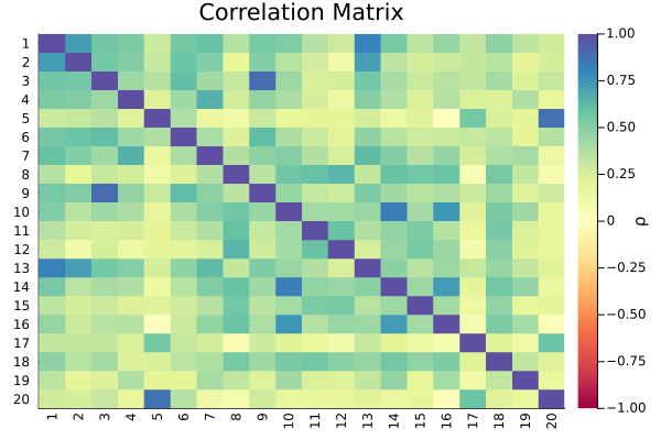
plot_correlation(X::MatNum, nx::AbstractVector = 1:size(X, 1); kwargs...) -> Plot
plot_correlation(pr::AbstractPriorResult, nx = 1:size(pr.sigma,1); kwargs...) -> Plot
plot_correlation(pr::AbstractPriorResult, rd::ReturnsResult; kwargs...) -> Plot
plot_correlation(res::OptimisationResult[, rd]; kwargs...) -> Plot
plot_correlation(pred::PredictionResult[, rd]; kwargs...) -> Plot
Standalone correlation (or covariance) heatmap without clustering or dendrograms.
plot_drawdowns(
    w::ArrNum,
    X::MatNum,
    fees::Option{<:Fees} = nothing;
    slv::Option{<:Slv_VecSlv} = nothing,
    ts::AbstractVector = 1:size(X, 1),
    compound::Bool = false,
    alpha::Number = 0.05,
    kappa::Number = 0.3,
    rw = nothing,
    kwargs...
) -> Plot
plot_drawdowns(w, rd::ReturnsResult, fees = nothing; slv, compound, alpha, kappa, rw, kwargs...) -> Plot
plot_drawdowns(res::OptimisationResult, rd; slv, compound, alpha, kappa, rw, kwargs...) -> Plot
plot_drawdowns(pred; slv, compound, alpha, kappa, rw, kwargs...) -> Plot
plot_drawdowns(mpred::MultiPeriodPredictionResult; slv, compound, alpha, kappa, rw, kwargs...) -> Plot
plot_drawdowns(ppred::PopulationPredictionResult; slv, compound, alpha, kappa, rw, kwargs...) -> Plot
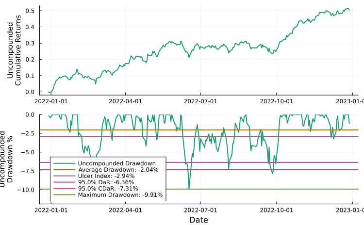
Plot portfolio drawdown over time.
plot_efficient_frontier(
    res_vec::AbstractVector{<:OptimisationResult},
    pr::Pr_RR;
    x::BaseRM_VecBaseRM = Variance(),
    y::BaseRM_VecBaseRM = ExpectedReturn(),
    c::BaseRM_VecBaseRM = ExpectedReturnRiskRatio(; rk=x, rt=ArithmeticReturn(), rf=0),
    slv::Option{<:Slv_VecSlv} = nothing,
    fees::Option{<:Fees} = nothing,
    min_risk::Bool = true,
    max_score::Bool = true,
    factory::Bool = true,
    kwargs...
) -> Plot
plot_efficient_frontier(res_vec, rd::ReturnsResult; kwargs...) -> Plot
plot_efficient_frontier(w::VecVecNum, pr::Pr_RR; x, y, c, slv, fees, min_risk, max_score, factory, kwargs...) -> Plot
plot_efficient_frontier(res::OptimisationResult, pr::Pr_RR; fees, kwargs...) -> Plot
plot_efficient_frontier(res::OptimisationResult, rd::ReturnsResult; kwargs...) -> Plot
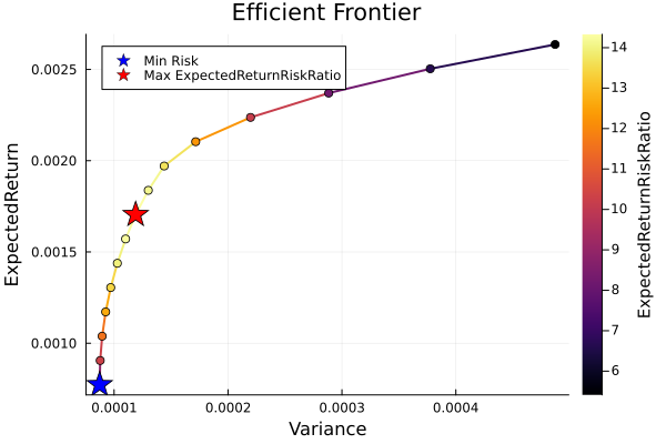
Sort a collection of portfolio results by risk (x), connect them with a line to trace the efficient frontier, and optionally annotate the minimum-risk and maximum-score portfolios.
plot_performance_summary(ps::PerformanceSummaryResult; kwargs...) -> Plot
plot_performance_summary(
    w::ArrNum,
    X::MatNum,
    fees::Option{<:Fees} = nothing;
    periods_per_year::Number = 252,
    alpha::Number = 0.05,
    compound::Bool = false,
    kwargs...
) -> Plot
plot_performance_summary(ret::VecNum; periods_per_year, alpha, compound, kwargs...) -> Plot
plot_performance_summary(w, rd::ReturnsResult, fees = nothing; alpha, compound, kwargs...) -> Plot
plot_performance_summary(res::OptimisationResult, rd; alpha, compound, kwargs...) -> Plot
plot_performance_summary(pred; alpha, compound, kwargs...) -> Plot
plot_performance_summary(mpred::MultiPeriodPredictionResult; alpha, compound, kwargs...) -> Plot
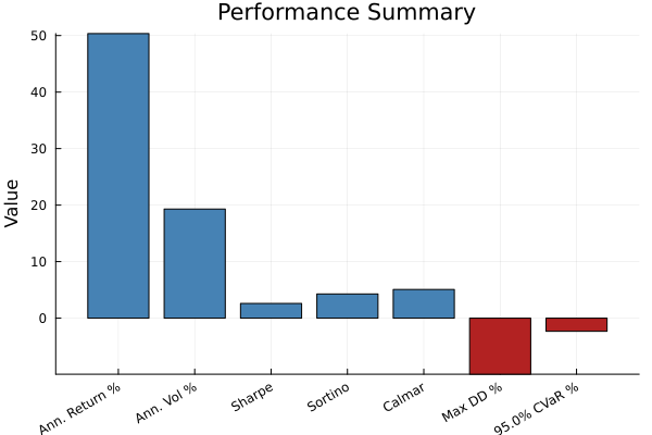
Bar chart of annualised portfolio performance metrics: annualised return, annualised volatility, Sharpe ratio, Sortino ratio, Calmar ratio, maximum drawdown %, and CVaR %.
plot_portfolio_cumulative_returns(
    w::VecNum_VecVecNum,
    X::MatNum,
    fees::Option{<:Fees} = nothing;
    ts::AbstractVector = 1:size(X, 1),
    compound::Bool = false,
    kwargs...
) -> Plot
plot_portfolio_cumulative_returns(
    w::VecNum_VecVecNum,
    pr::Pr_RR,
    fees::Option{<:Fees} = nothing;
    ts::AbstractVector = 1:size(pr.X, 1),
    compound::Bool = false,
    kwargs...
) -> Plot
plot_portfolio_cumulative_returns(
    res::OptimisationResult,
    pr::Pr_RR;
    fees::Option{<:Fees} = nothing,
    compound::Bool = false,
    kwargs...
) -> Plot
plot_portfolio_cumulative_returns(
    res::OptimisationResult;
    fees::Option{<:Fees} = nothing,
    compound::Bool = false,
    kwargs...
) -> Plot
plot_portfolio_cumulative_returns(
    pred::Union{
                    <:PredictionResult,
                    <:MultiPeriodPredictionResult,
                    <:PopulationPredictionResult
                };
    compound::Bool = false,
    kwargs...
) -> Plot
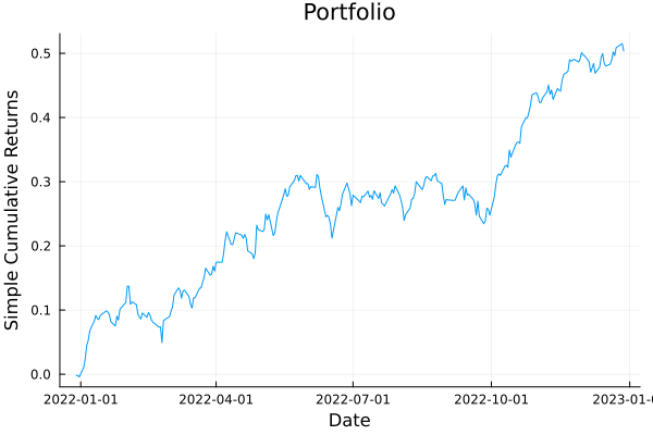
Plot the cumulative returns of a portfolio.
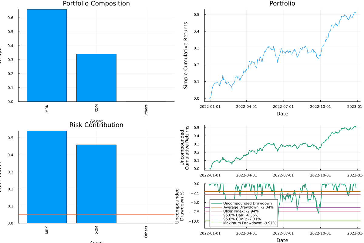
plot_portfolio_dashboard(
    res::OptimisationResult,
    rd::Pr_RR;
    ts = 1:size(rd.X, 1),
    nx = 1:size(rd.X, 2),
    r::AbstractBaseRiskMeasure = Variance(),
    slv::Option{<:Slv_VecSlv} = nothing,
    compound::Bool = false,
    N::Option{<:Number} = nothing,
    delta::Number = 1e-6,
    marginal::Bool = false,
    percentage::Bool = false,
    alpha::Number = 0.05,
    kappa::Number = 0.3,
    rw = nothing,
    kwargs...
) -> Plot
Four-panel composite plot for a single optimisation result:
plot_prior(
    pr::AbstractPriorResult,
    nx::AbstractVector = 1:length(pr.mu);
    N::Option{<:Number} = nothing,
    kwargs...
) -> Plot
plot_prior(pr::AbstractPriorResult, rd::ReturnsResult; N, kwargs...) -> Plot
plot_prior(res::OptimisationResult[, rd]; N, kwargs...) -> Plot
plot_prior(pred::PredictionResult[, rd]; N, kwargs...) -> Plot
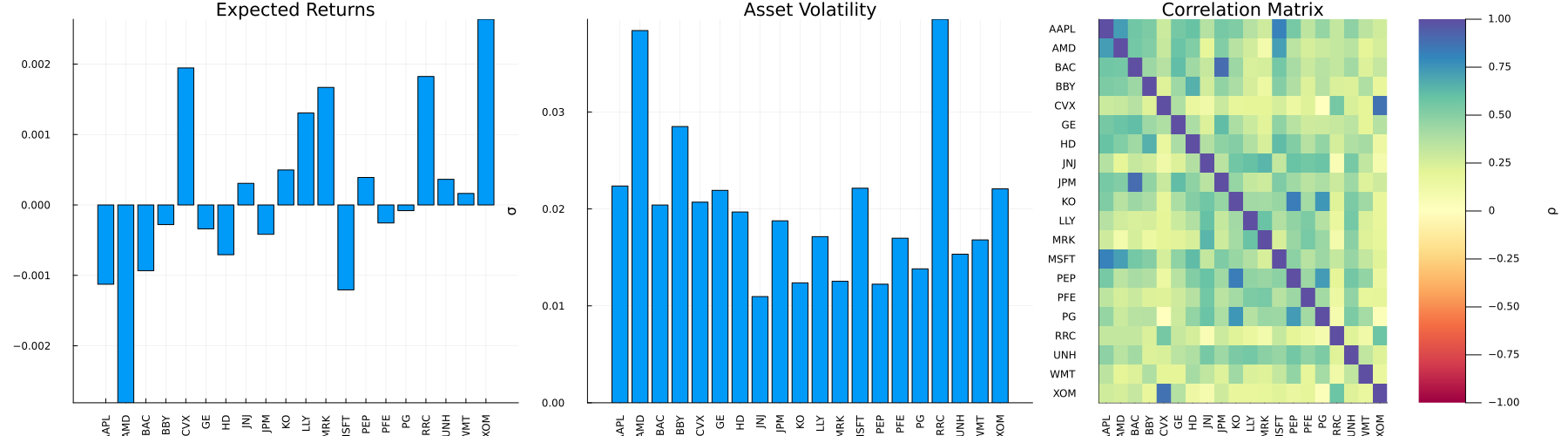
Three-panel composite plot summarising a prior result:
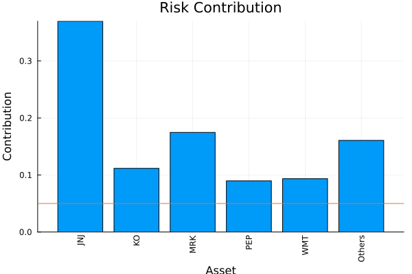
plot_risk_contribution(
    r::BaseRM_VecBaseRM,
    w::VecNum,
    X::MatNum_Pr,
    fees::Option{<:Fees} = nothing;
    nx::AbstractVector = 1:length(w),
    delta::Number = 1e-6,
    marginal::Bool = false,
    percentage::Bool = false,
    N::Option{<:Number} = nothing,
    sca::Scalariser = SumScalariser(),
    kwargs...
) -> Plot
plot_risk_contribution(r, w, rd::ReturnsResult, fees = nothing; delta, marginal, percentage, N, sca, kwargs...) -> Plot
plot_risk_contribution(r, res::OptimisationResult, rd; delta, marginal, percentage, N, sca, kwargs...) -> Plot
plot_risk_contribution(r, res::OptimisationResult, pr; nx, delta, marginal, percentage, N, sca, kwargs...) -> Plot
Plot per-asset risk contribution as a bar chart.
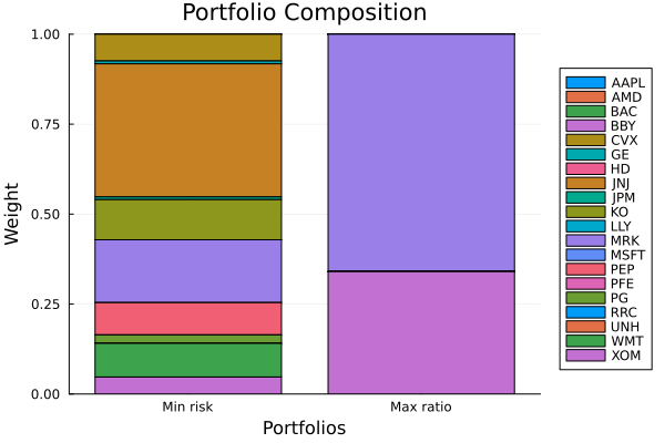
plot_stacked_bar_composition(
    w::VecNum_VecVecNum,
    nx::AbstractVector = 1:size(w, 1);
    kwargs...
) -> Plot
plot_stacked_bar_composition(res_vec::AbstractVector{<:OptimisationResult}, rd; kwargs...) -> Plot
Plot portfolio composition as a stacked bar chart.