The source files can be found in user_guide/.
Constraints and costs
A real mandate has constraints. You cap the weight of one asset, hold a sector inside a band, limit how much you trade at each rebalance, and pay fees. In PortfolioOptimisers.jl these are keywords of the JuMPOptimiser. The JuMPOptimiser holds the constraints and the costs, and the optimiser that takes it, such as MeanRisk, holds the objective. This page shows the common ones with one minimal call each. For the others, see the constraints and costs examples.
We compute one empirical prior. Every call but the factor call uses it, and every call but the last two minimises the risk. You can then compare the portfolio under each constraint with the same base portfolio.
using PortfolioOptimisers, CSV, TimeSeries, DataFrames, PrettyTables, Clarabel, StatsPlots, GraphRecipesresfmt = (v, i, j) -> begin return if j == 1 v else isa(v, AbstractFloat) ? "$(round(v*100, digits=3)) %" : v endend;X = TimeArray(CSV.File(joinpath(@__DIR__, "../examples/SP500.csv.gz")); timestamp = :Date)[(end - 252):end]rd = prices_to_returns(X)pr = prior(EmpiricalPrior(), rd)slv = Solver(; name = :clarabel, solver = Clarabel.Optimizer, settings = Dict("verbose" => false), check_sol = (; allow_local = true, allow_almost = true))res_base = optimise(MeanRisk(; obj = MinimumRisk(), opt = JuMPOptimiser(; pe = pr, slv = slv)))MeanRiskResult
jr ┼ JuMPOptimisationResult
│ pa ┼ ProcessedJuMPOptimiserAttributes
│ │ pr ┼ LowOrderPrior
│ │ │ X ┼ 252×20 Matrix{Float64}
│ │ │ o_X ┼ nothing
│ │ │ mu ┼ 20-element Vector{Float64}
│ │ │ sigma ┼ 20×20 Matrix{Float64}
│ │ │ chol ┼ nothing
│ │ │ w ┼ nothing
│ │ │ ens ┼ nothing
│ │ │ kld ┼ nothing
│ │ │ ow ┼ nothing
│ │ │ rr ┼ nothing
│ │ │ fpr ┴ nothing
│ │ wb ┼ WeightBounds
│ │ │ lb ┼ 20-element StepRangeLen{Float64, Base.TwicePrecision{Float64}, Base.TwicePrecision{Float64}, Int64}
│ │ │ ub ┴ 20-element StepRangeLen{Float64, Base.TwicePrecision{Float64}, Base.TwicePrecision{Float64}, Int64}
│ │ lt ┼ nothing
│ │ st ┼ nothing
│ │ lcsr ┼ nothing
│ │ ctr ┼ nothing
│ │ gcardr ┼ nothing
│ │ sgcardr ┼ nothing
│ │ smtx ┼ nothing
│ │ sgmtx ┼ nothing
│ │ slt ┼ nothing
│ │ sst ┼ nothing
│ │ sglt ┼ nothing
│ │ sgst ┼ nothing
│ │ tn ┼ nothing
│ │ fees ┼ nothing
│ │ plr ┼ nothing
│ │ ret ┼ ArithmeticReturn
│ │ │ settings ┼ JuMPReturnsSettings
│ │ │ │ scale ┼ Float64: 1.0
│ │ │ │ lb ┼ nothing
│ │ │ │ rte ┼ Bool: true
│ │ │ │ fee ┼ Bool: true
│ │ │ │ mic ┴ Bool: true
│ │ │ ucs ┼ nothing
│ │ │ mu ┴ 20-element Vector{Float64}
│ │ sca ┼ SumScalariser()
│ │ imsk ┴ nothing
│ retcode ┼ OptimisationSuccess
│ │ res ┴ Dict{Any, Any}: Dict{Any, Any}()
│ sol ┼ JuMPOptimisationSolution
│ │ w ┴ 20-element Vector{Float64}
│ model ┼ A JuMP Model
│ │ ├ solver: Clarabel
│ │ ├ objective_sense: MIN_SENSE
│ │ │ └ objective_function_type: QuadExpr
│ │ ├ num_variables: 21
│ │ ├ num_constraints: 4
│ │ │ ├ AffExpr in MOI.EqualTo{Float64}: 1
│ │ │ ├ Vector{AffExpr} in MOI.Nonnegatives: 1
│ │ │ ├ Vector{AffExpr} in MOI.Nonpositives: 1
│ │ │ └ Vector{AffExpr} in MOI.SecondOrderCone: 1
│ │ └ Names registered in the model
│ │ └ :G, :T, :bgt, :cdev_soc_1, :dev_1, :k, :lw, :obj_expr, :ret, :ret_1, :ret_vec, :risk, :risk_minimised, :risk_vec, :sc, :so, :variance_flag, :variance_risk_1, :w, :w_gross_ub, :w_lb, :w_ub
r ┼ Variance
│ settings ┼ RiskMeasureSettings
│ │ scale ┼ Float64: 1.0
│ │ ub ┼ nothing
│ │ rke ┴ Bool: true
│ sigma ┼ 20×20 Matrix{Float64}
│ chol ┼ nothing
│ rc ┼ nothing
│ alg ┴ SquaredSOCRiskExpr()
fb ┴ nothing
1. Weight bounds
WeightBounds sets a lower and an upper bound on the weight of each asset, through the wb keyword. The default is lb = 0 and ub = 1, a long-only portfolio. A lower ub spreads the weight over more assets, because no asset can hold more than the bound.
res_cap = optimise(MeanRisk(; obj = MinimumRisk(), opt = JuMPOptimiser(; pe = pr, slv = slv, wb = WeightBounds(; lb = 0.0, ub = 0.10))))MeanRiskResult
jr ┼ JuMPOptimisationResult
│ pa ┼ ProcessedJuMPOptimiserAttributes
│ │ pr ┼ LowOrderPrior
│ │ │ X ┼ 252×20 Matrix{Float64}
│ │ │ o_X ┼ nothing
│ │ │ mu ┼ 20-element Vector{Float64}
│ │ │ sigma ┼ 20×20 Matrix{Float64}
│ │ │ chol ┼ nothing
│ │ │ w ┼ nothing
│ │ │ ens ┼ nothing
│ │ │ kld ┼ nothing
│ │ │ ow ┼ nothing
│ │ │ rr ┼ nothing
│ │ │ fpr ┴ nothing
│ │ wb ┼ WeightBounds
│ │ │ lb ┼ 20-element StepRangeLen{Float64, Base.TwicePrecision{Float64}, Base.TwicePrecision{Float64}, Int64}
│ │ │ ub ┴ 20-element StepRangeLen{Float64, Base.TwicePrecision{Float64}, Base.TwicePrecision{Float64}, Int64}
│ │ lt ┼ nothing
│ │ st ┼ nothing
│ │ lcsr ┼ nothing
│ │ ctr ┼ nothing
│ │ gcardr ┼ nothing
│ │ sgcardr ┼ nothing
│ │ smtx ┼ nothing
│ │ sgmtx ┼ nothing
│ │ slt ┼ nothing
│ │ sst ┼ nothing
│ │ sglt ┼ nothing
│ │ sgst ┼ nothing
│ │ tn ┼ nothing
│ │ fees ┼ nothing
│ │ plr ┼ nothing
│ │ ret ┼ ArithmeticReturn
│ │ │ settings ┼ JuMPReturnsSettings
│ │ │ │ scale ┼ Float64: 1.0
│ │ │ │ lb ┼ nothing
│ │ │ │ rte ┼ Bool: true
│ │ │ │ fee ┼ Bool: true
│ │ │ │ mic ┴ Bool: true
│ │ │ ucs ┼ nothing
│ │ │ mu ┴ 20-element Vector{Float64}
│ │ sca ┼ SumScalariser()
│ │ imsk ┴ nothing
│ retcode ┼ OptimisationSuccess
│ │ res ┴ Dict{Any, Any}: Dict{Any, Any}()
│ sol ┼ JuMPOptimisationSolution
│ │ w ┴ 20-element Vector{Float64}
│ model ┼ A JuMP Model
│ │ ├ solver: Clarabel
│ │ ├ objective_sense: MIN_SENSE
│ │ │ └ objective_function_type: QuadExpr
│ │ ├ num_variables: 21
│ │ ├ num_constraints: 4
│ │ │ ├ AffExpr in MOI.EqualTo{Float64}: 1
│ │ │ ├ Vector{AffExpr} in MOI.Nonnegatives: 1
│ │ │ ├ Vector{AffExpr} in MOI.Nonpositives: 1
│ │ │ └ Vector{AffExpr} in MOI.SecondOrderCone: 1
│ │ └ Names registered in the model
│ │ └ :G, :T, :bgt, :cdev_soc_1, :dev_1, :k, :lw, :obj_expr, :ret, :ret_1, :ret_vec, :risk, :risk_minimised, :risk_vec, :sc, :so, :variance_flag, :variance_risk_1, :w, :w_gross_ub, :w_lb, :w_ub
r ┼ Variance
│ settings ┼ RiskMeasureSettings
│ │ scale ┼ Float64: 1.0
│ │ ub ┼ nothing
│ │ rke ┴ Bool: true
│ sigma ┼ 20×20 Matrix{Float64}
│ chol ┼ nothing
│ rc ┼ nothing
│ alg ┴ SquaredSOCRiskExpr()
fb ┴ nothing
The budget, the sum of the weights, is the bgt keyword, 1.0 by default. With BudgetRange and a separate short budget sbgt, you can build a long-short portfolio or a leveraged portfolio. See Budget Constraints.
2. Linear and group constraints
You write a group constraint or a linear constraint as a string over a UniverseSets, and you pass it to lcse in a LinearConstraintEstimator. Views use the same syntax. Name a group, then bound it. We require the tech group to hold at least 15% of the weight. The minimum-risk portfolio gives it almost none.
sets = UniverseSets(; dict = Dict("nx" => rd.nx, "tech" => ["AAPL", "AMD", "MSFT"]))res_grp = optimise(MeanRisk(; obj = MinimumRisk(), opt = JuMPOptimiser(; pe = pr, slv = slv, sets = sets, lcse = LinearConstraintEstimator(; val = ["tech >= 0.15"]))))MeanRiskResult
jr ┼ JuMPOptimisationResult
│ pa ┼ ProcessedJuMPOptimiserAttributes
│ │ pr ┼ LowOrderPrior
│ │ │ X ┼ 252×20 Matrix{Float64}
│ │ │ o_X ┼ nothing
│ │ │ mu ┼ 20-element Vector{Float64}
│ │ │ sigma ┼ 20×20 Matrix{Float64}
│ │ │ chol ┼ nothing
│ │ │ w ┼ nothing
│ │ │ ens ┼ nothing
│ │ │ kld ┼ nothing
│ │ │ ow ┼ nothing
│ │ │ rr ┼ nothing
│ │ │ fpr ┴ nothing
│ │ wb ┼ WeightBounds
│ │ │ lb ┼ 20-element StepRangeLen{Float64, Base.TwicePrecision{Float64}, Base.TwicePrecision{Float64}, Int64}
│ │ │ ub ┴ 20-element StepRangeLen{Float64, Base.TwicePrecision{Float64}, Base.TwicePrecision{Float64}, Int64}
│ │ lt ┼ nothing
│ │ st ┼ nothing
│ │ lcsr ┼ LinearConstraint
│ │ │ ineq ┼ PartialLinearConstraint
│ │ │ │ A ┼ 1×20 LinearAlgebra.Transpose{Float64, Matrix{Float64}}
│ │ │ │ B ┴ Vector{Float64}: [-0.15]
│ │ │ eq ┴ nothing
│ │ ctr ┼ nothing
│ │ gcardr ┼ nothing
│ │ sgcardr ┼ nothing
│ │ smtx ┼ nothing
│ │ sgmtx ┼ nothing
│ │ slt ┼ nothing
│ │ sst ┼ nothing
│ │ sglt ┼ nothing
│ │ sgst ┼ nothing
│ │ tn ┼ nothing
│ │ fees ┼ nothing
│ │ plr ┼ nothing
│ │ ret ┼ ArithmeticReturn
│ │ │ settings ┼ JuMPReturnsSettings
│ │ │ │ scale ┼ Float64: 1.0
│ │ │ │ lb ┼ nothing
│ │ │ │ rte ┼ Bool: true
│ │ │ │ fee ┼ Bool: true
│ │ │ │ mic ┴ Bool: true
│ │ │ ucs ┼ nothing
│ │ │ mu ┴ 20-element Vector{Float64}
│ │ sca ┼ SumScalariser()
│ │ imsk ┴ nothing
│ retcode ┼ OptimisationSuccess
│ │ res ┴ Dict{Any, Any}: Dict{Any, Any}()
│ sol ┼ JuMPOptimisationSolution
│ │ w ┴ 20-element Vector{Float64}
│ model ┼ A JuMP Model
│ │ ├ solver: Clarabel
│ │ ├ objective_sense: MIN_SENSE
│ │ │ └ objective_function_type: QuadExpr
│ │ ├ num_variables: 21
│ │ ├ num_constraints: 5
│ │ │ ├ AffExpr in MOI.EqualTo{Float64}: 1
│ │ │ ├ Vector{AffExpr} in MOI.Nonnegatives: 1
│ │ │ ├ Vector{AffExpr} in MOI.Nonpositives: 2
│ │ │ └ Vector{AffExpr} in MOI.SecondOrderCone: 1
│ │ └ Names registered in the model
│ │ └ :G, :T, :bgt, :cdev_soc_1, :dev_1, :k, :lcs_ineq_1, :lw, :obj_expr, :ret, :ret_1, :ret_vec, :risk, :risk_minimised, :risk_vec, :sc, :so, :variance_flag, :variance_risk_1, :w, :w_gross_ub, :w_lb, :w_ub
r ┼ Variance
│ settings ┼ RiskMeasureSettings
│ │ scale ┼ Float64: 1.0
│ │ ub ┼ nothing
│ │ rke ┴ Bool: true
│ sigma ┼ 20×20 Matrix{Float64}
│ chol ┼ nothing
│ rc ┼ nothing
│ alg ┴ SquaredSOCRiskExpr()
fb ┴ nothing
The same lcse takes a bound on one asset, such as "AAPL <= 0.1", and a bound between two assets, such as "MSFT >= AMD". For constraints built from the hierarchy of the assets, see Phylogeny and Centrality.
3. Factor exposure constraints
A mandate often names factors and not assets, as in "at most 10% momentum" or "no net exposure to value". Such a constraint bounds the factor exposures of the portfolio, w_f = Mᵀw, where M is the matrix of loadings that a factor model computes.
Put a LinearConstraintEstimator in an ExposureConstraintEstimator, and set its space keyword to FactorSpace. The keyword has no default. The names in the constraint must be factor names of the loadings. For a time-series regression, these are the names that a UniverseSets holds under tfkey, "nf" by default. When the estimator builds the constraint, it multiplies each row by the loadings. The optimiser then receives an ordinary constraint on the asset weights, which you can combine with every other constraint on this page.
The constraint needs loadings, and the loadings need factor data. prices_to_returns takes no factor prices, so we give them to price_ingestion as F. By default the loadings come from the prior, so the prior must be a FactorPrior and not an EmpiricalPrior. If the prior has no loadings, the constraint throws an error, and it does not drop the row. FactorSpace(; re = <a fitted Regression>) fixes the loadings. FactorSpace(; re = StepwiseRegression()) fits them when the prior has none, so the constraint works on any prior. The factor exposure example gives the order in which these sources apply.
Fac = TimeArray(CSV.File(joinpath(@__DIR__, "../examples/Factors.csv.gz")); timestamp = :Date)[(end - 252):end]rd_f = prices_to_returns(price_ingestion(PriceIngestion(), X; F = Fac))sets_f = UniverseSets(; dict = Dict("nx" => rd_f.nx, "nf" => rd_f.nf))res_fac = optimise(MeanRisk(; obj = MinimumRisk(), opt = JuMPOptimiser(; pe = FactorPrior(), slv = slv, sets = sets_f, lcse = ExposureConstraintEstimator(; lce = LinearConstraintEstimator(; val = "MTUM >= 0.2"), space = FactorSpace()))), rd_f)MeanRiskResult
jr ┼ JuMPOptimisationResult
│ pa ┼ ProcessedJuMPOptimiserAttributes
│ │ pr ┼ LowOrderPrior
│ │ │ X ┼ 252×20 Matrix{Float64}
│ │ │ o_X ┼ 252×20 Matrix{Float64}
│ │ │ mu ┼ 20-element Vector{Float64}
│ │ │ sigma ┼ 20×20 Matrix{Float64}
│ │ │ chol ┼ 25×20 LinearAlgebra.Transpose{Float64, Matrix{Float64}}
│ │ │ w ┼ nothing
│ │ │ ens ┼ nothing
│ │ │ kld ┼ nothing
│ │ │ ow ┼ nothing
│ │ │ rr ┼ Regression
│ │ │ │ M ┼ 20×5 SubArray{Float64, 2, Matrix{Float64}, Tuple{Base.Slice{Base.OneTo{Int64}}, UnitRange{Int64}}, true}
│ │ │ │ L ┼ 20×5 SubArray{Float64, 2, Matrix{Float64}, Tuple{Base.Slice{Base.OneTo{Int64}}, UnitRange{Int64}}, true}
│ │ │ │ b ┼ 20-element SubArray{Float64, 1, Matrix{Float64}, Tuple{Base.Slice{Base.OneTo{Int64}}, Int64}, true}
│ │ │ │ esigma ┼ 20-element Vector{Float64}
│ │ │ │ edof ┼ 20-element Vector{Int64}
│ │ │ │ ediv ┴ 20-element Vector{Int64}
│ │ │ fpr ┼ LowOrderPrior
│ │ │ │ X ┼ 252×5 Matrix{Float64}
│ │ │ │ o_X ┼ nothing
│ │ │ │ mu ┼ Vector{Float64}: [-0.0007221367902182357, -0.0008384535501032073, -0.0006253517821839465, -0.0003358529620217417, -0.000559091885073412]
│ │ │ │ sigma ┼ 5×5 Matrix{Float64}
│ │ │ │ chol ┼ nothing
│ │ │ │ w ┼ nothing
│ │ │ │ ens ┼ nothing
│ │ │ │ kld ┼ nothing
│ │ │ │ ow ┼ nothing
│ │ │ │ rr ┼ nothing
│ │ │ │ fpr ┴ nothing
│ │ wb ┼ WeightBounds
│ │ │ lb ┼ 20-element StepRangeLen{Float64, Base.TwicePrecision{Float64}, Base.TwicePrecision{Float64}, Int64}
│ │ │ ub ┴ 20-element StepRangeLen{Float64, Base.TwicePrecision{Float64}, Base.TwicePrecision{Float64}, Int64}
│ │ lt ┼ nothing
│ │ st ┼ nothing
│ │ lcsr ┼ LinearConstraint
│ │ │ ineq ┼ PartialLinearConstraint
│ │ │ │ A ┼ 1×20 LinearAlgebra.Transpose{Float64, Matrix{Float64}}
│ │ │ │ B ┴ Vector{Float64}: [-0.2]
│ │ │ eq ┴ nothing
│ │ ctr ┼ nothing
│ │ gcardr ┼ nothing
│ │ sgcardr ┼ nothing
│ │ smtx ┼ nothing
│ │ sgmtx ┼ nothing
│ │ slt ┼ nothing
│ │ sst ┼ nothing
│ │ sglt ┼ nothing
│ │ sgst ┼ nothing
│ │ tn ┼ nothing
│ │ fees ┼ nothing
│ │ plr ┼ nothing
│ │ ret ┼ ArithmeticReturn
│ │ │ settings ┼ JuMPReturnsSettings
│ │ │ │ scale ┼ Float64: 1.0
│ │ │ │ lb ┼ nothing
│ │ │ │ rte ┼ Bool: true
│ │ │ │ fee ┼ Bool: true
│ │ │ │ mic ┴ Bool: true
│ │ │ ucs ┼ nothing
│ │ │ mu ┴ 20-element Vector{Float64}
│ │ sca ┼ SumScalariser()
│ │ imsk ┴ nothing
│ retcode ┼ OptimisationSuccess
│ │ res ┴ Dict{Any, Any}: Dict{Any, Any}()
│ sol ┼ JuMPOptimisationSolution
│ │ w ┴ 20-element Vector{Float64}
│ model ┼ A JuMP Model
│ │ ├ solver: Clarabel
│ │ ├ objective_sense: MIN_SENSE
│ │ │ └ objective_function_type: QuadExpr
│ │ ├ num_variables: 21
│ │ ├ num_constraints: 5
│ │ │ ├ AffExpr in MOI.EqualTo{Float64}: 1
│ │ │ ├ Vector{AffExpr} in MOI.Nonnegatives: 1
│ │ │ ├ Vector{AffExpr} in MOI.Nonpositives: 2
│ │ │ └ Vector{AffExpr} in MOI.SecondOrderCone: 1
│ │ └ Names registered in the model
│ │ └ :G, :T, :bgt, :cdev_soc_1, :dev_1, :k, :lcs_ineq_1, :lw, :obj_expr, :ret, :ret_1, :ret_vec, :risk, :risk_minimised, :risk_vec, :sc, :so, :variance_flag, :variance_risk_1, :w, :w_gross_ub, :w_lb, :w_ub
r ┼ Variance
│ settings ┼ RiskMeasureSettings
│ │ scale ┼ Float64: 1.0
│ │ ub ┼ nothing
│ │ rke ┴ Bool: true
│ sigma ┼ 20×20 Matrix{Float64}
│ chol ┼ 25×20 LinearAlgebra.Transpose{Float64, Matrix{Float64}}
│ rc ┼ nothing
│ alg ┴ SquaredSOCRiskExpr()
fb ┴ nothing
We compute the factor exposures of the result with the loadings on its prior, which are the loadings that the optimiser used. The MTUM row shows the floor of the constraint.
pretty_table(DataFrame("Factor" => rd_f.nf, "Exposure" => transpose(res_fac.pa.pr.rr.M) * res_fac.w); formatters = [resfmt], title = "Realised factor exposures")Realised factor exposures
┌────────┬───────────┐
│ Factor │ Exposure │
│ String │ Float64 │
├────────┼───────────┤
│ MTUM │ 20.0 % │
│ QUAL │ -35.285 % │
│ SIZE │ -48.777 % │
│ USMV │ 96.28 % │
│ VLUE │ 49.392 % │
└────────┴───────────┘Pass the prior estimator, not a computed prior. Then the optimiser builds the constraint again inside each cross-validation fold, with the loadings that the fold fitted. A row that you compute by hand once does not match the loadings of the later folds, and the factor exposure example measures how far it moves. That page also covers groups of factors, factor rows mixed with asset rows, and the constraints that have no factor form.
A constraint has a factor form only if it is a linear row in w. Cardinality, thresholds, turnover, tracking error and fees have none. Weight bounds have none either, because wb takes a box on each asset and no linear rows. To bound a factor exposure from both sides, write the two rows through lcse. To track a factor, you need no factor form. ReturnsTracking takes the return series of a benchmark, and the return series of a factor is a column of the factor matrix.
4. Turnover
Trading limits and costs are keywords too. Turnover (tn) bounds how far the weight of each asset can move from a reference portfolio w, which is usually the portfolio that you hold. val is the largest change for each asset. We use the equal-weighted portfolio as the portfolio that you hold, and we bound the change of each asset at 0.02.
w_held = fill(inv(length(rd.nx)), length(rd.nx))res_tn = optimise(MeanRisk(; obj = MinimumRisk(), opt = JuMPOptimiser(; pe = pr, slv = slv, tn = Turnover(; w = w_held, val = 0.02))))MeanRiskResult
jr ┼ JuMPOptimisationResult
│ pa ┼ ProcessedJuMPOptimiserAttributes
│ │ pr ┼ LowOrderPrior
│ │ │ X ┼ 252×20 Matrix{Float64}
│ │ │ o_X ┼ nothing
│ │ │ mu ┼ 20-element Vector{Float64}
│ │ │ sigma ┼ 20×20 Matrix{Float64}
│ │ │ chol ┼ nothing
│ │ │ w ┼ nothing
│ │ │ ens ┼ nothing
│ │ │ kld ┼ nothing
│ │ │ ow ┼ nothing
│ │ │ rr ┼ nothing
│ │ │ fpr ┴ nothing
│ │ wb ┼ WeightBounds
│ │ │ lb ┼ 20-element StepRangeLen{Float64, Base.TwicePrecision{Float64}, Base.TwicePrecision{Float64}, Int64}
│ │ │ ub ┴ 20-element StepRangeLen{Float64, Base.TwicePrecision{Float64}, Base.TwicePrecision{Float64}, Int64}
│ │ lt ┼ nothing
│ │ st ┼ nothing
│ │ lcsr ┼ nothing
│ │ ctr ┼ nothing
│ │ gcardr ┼ nothing
│ │ sgcardr ┼ nothing
│ │ smtx ┼ nothing
│ │ sgmtx ┼ nothing
│ │ slt ┼ nothing
│ │ sst ┼ nothing
│ │ sglt ┼ nothing
│ │ sgst ┼ nothing
│ │ tn ┼ Turnover
│ │ │ w ┼ 20-element Vector{Float64}
│ │ │ val ┼ Float64: 0.02
│ │ │ fixed ┴ Bool: false
│ │ fees ┼ nothing
│ │ plr ┼ nothing
│ │ ret ┼ ArithmeticReturn
│ │ │ settings ┼ JuMPReturnsSettings
│ │ │ │ scale ┼ Float64: 1.0
│ │ │ │ lb ┼ nothing
│ │ │ │ rte ┼ Bool: true
│ │ │ │ fee ┼ Bool: true
│ │ │ │ mic ┴ Bool: true
│ │ │ ucs ┼ nothing
│ │ │ mu ┴ 20-element Vector{Float64}
│ │ sca ┼ SumScalariser()
│ │ imsk ┴ nothing
│ retcode ┼ OptimisationSuccess
│ │ res ┴ Dict{Any, Any}: Dict{Any, Any}()
│ sol ┼ JuMPOptimisationSolution
│ │ w ┴ 20-element Vector{Float64}
│ model ┼ A JuMP Model
│ │ ├ solver: Clarabel
│ │ ├ objective_sense: MIN_SENSE
│ │ │ └ objective_function_type: QuadExpr
│ │ ├ num_variables: 41
│ │ ├ num_constraints: 25
│ │ │ ├ AffExpr in MOI.EqualTo{Float64}: 1
│ │ │ ├ Vector{AffExpr} in MOI.Nonnegatives: 1
│ │ │ ├ Vector{AffExpr} in MOI.Nonpositives: 2
│ │ │ ├ Vector{AffExpr} in MOI.NormOneCone: 20
│ │ │ └ Vector{AffExpr} in MOI.SecondOrderCone: 1
│ │ └ Names registered in the model
│ │ └ :G, :T, :bgt, :cdev_soc_1, :ctn_1, :ctn_noc_1, :dev_1, :k, :lw, :obj_expr, :ret, :ret_1, :ret_vec, :risk, :risk_minimised, :risk_vec, :sc, :so, :t_tn_1, :tn_1, :variance_flag, :variance_risk_1, :w, :w_gross_ub, :w_lb, :w_ub
r ┼ Variance
│ settings ┼ RiskMeasureSettings
│ │ scale ┼ Float64: 1.0
│ │ ub ┼ nothing
│ │ rke ┴ Bool: true
│ sigma ┼ 20×20 Matrix{Float64}
│ chol ┼ nothing
│ rc ┼ nothing
│ alg ┴ SquaredSOCRiskExpr()
fb ┴ nothing
The reference holds 5% in each of the 20 assets, so each weight of the result stays between 3% and 7%. The base portfolio holds about 37% in one asset, and the bound keeps that asset at 7% or less. The Turnover column of the table at the end shows the result. A larger val lets the result move further from the reference, towards the base portfolio. If the reference is the optimum of the same problem, the bound changes almost nothing, because the optimum is already inside it.
5. Fees
Fees (fees) charges a fee in each period on the positions that you hold, at one rate on the long weights and at another on the short weights, with optional fixed fees. It can also charge a fee on the traded weights. The optimiser subtracts the fees from the expected return, which a return objective and a return floor use, and from the return of each period, which a risk measure such as ConditionalValueatRisk uses. The variance, the default risk measure of MeanRisk, uses neither, and a fee does not change the MinimumRisk portfolios of this page. The minimal form sets l, the rate on the long weights. We maximise the ratio of return to risk with MaximumRatio two times, first with no fee and then with a rate of 0.1% on the long weights. The two portfolios differ only by the fee.
res_ratio = optimise(MeanRisk(; obj = MaximumRatio(; rf = 4.2 / 100 / 252), opt = JuMPOptimiser(; pe = pr, slv = slv)))res_fee = optimise(MeanRisk(; obj = MaximumRatio(; rf = 4.2 / 100 / 252), opt = JuMPOptimiser(; pe = pr, slv = slv, fees = Fees(; l = 0.001))))MeanRiskResult
jr ┼ JuMPOptimisationResult
│ pa ┼ ProcessedJuMPOptimiserAttributes
│ │ pr ┼ LowOrderPrior
│ │ │ X ┼ 252×20 Matrix{Float64}
│ │ │ o_X ┼ nothing
│ │ │ mu ┼ 20-element Vector{Float64}
│ │ │ sigma ┼ 20×20 Matrix{Float64}
│ │ │ chol ┼ nothing
│ │ │ w ┼ nothing
│ │ │ ens ┼ nothing
│ │ │ kld ┼ nothing
│ │ │ ow ┼ nothing
│ │ │ rr ┼ nothing
│ │ │ fpr ┴ nothing
│ │ wb ┼ WeightBounds
│ │ │ lb ┼ 20-element StepRangeLen{Float64, Base.TwicePrecision{Float64}, Base.TwicePrecision{Float64}, Int64}
│ │ │ ub ┴ 20-element StepRangeLen{Float64, Base.TwicePrecision{Float64}, Base.TwicePrecision{Float64}, Int64}
│ │ lt ┼ nothing
│ │ st ┼ nothing
│ │ lcsr ┼ nothing
│ │ ctr ┼ nothing
│ │ gcardr ┼ nothing
│ │ sgcardr ┼ nothing
│ │ smtx ┼ nothing
│ │ sgmtx ┼ nothing
│ │ slt ┼ nothing
│ │ sst ┼ nothing
│ │ sglt ┼ nothing
│ │ sgst ┼ nothing
│ │ tn ┼ nothing
│ │ fees ┼ Fees
│ │ │ tn ┼ nothing
│ │ │ l ┼ Float64: 0.001
│ │ │ s ┼ nothing
│ │ │ fl ┼ nothing
│ │ │ fs ┼ nothing
│ │ │ lq ┼ nothing
│ │ │ flq ┼ nothing
│ │ │ fa ┼ nothing
│ │ │ kwargs ┴ @NamedTuple{atol::Float64}: (atol = 1.0e-8,)
│ │ plr ┼ nothing
│ │ ret ┼ ArithmeticReturn
│ │ │ settings ┼ JuMPReturnsSettings
│ │ │ │ scale ┼ Float64: 1.0
│ │ │ │ lb ┼ nothing
│ │ │ │ rte ┼ Bool: true
│ │ │ │ fee ┼ Bool: true
│ │ │ │ mic ┴ Bool: true
│ │ │ ucs ┼ nothing
│ │ │ mu ┴ 20-element Vector{Float64}
│ │ sca ┼ SumScalariser()
│ │ imsk ┴ nothing
│ retcode ┼ OptimisationSuccess
│ │ res ┴ Dict{Any, Any}: Dict{Any, Any}()
│ sol ┼ JuMPOptimisationSolution
│ │ w ┴ 20-element Vector{Float64}
│ model ┼ A JuMP Model
│ │ ├ solver: Clarabel
│ │ ├ objective_sense: MIN_SENSE
│ │ │ └ objective_function_type: QuadExpr
│ │ ├ num_variables: 22
│ │ ├ num_constraints: 6
│ │ │ ├ AffExpr in MOI.EqualTo{Float64}: 2
│ │ │ ├ Vector{AffExpr} in MOI.Nonnegatives: 1
│ │ │ ├ Vector{AffExpr} in MOI.Nonpositives: 1
│ │ │ ├ Vector{AffExpr} in MOI.SecondOrderCone: 1
│ │ │ └ VariableRef in MOI.GreaterThan{Float64}: 1
│ │ └ Names registered in the model
│ │ └ :G, :T, :bgt, :cdev_soc_1, :dev_1, :fee_fa, :fees, :fl, :k, :lw, :obj_expr, :ohf, :ret, :ret_1, :ret_vec, :risk, :risk_minimised, :risk_vec, :sc, :so, :sr_ret, :variance_flag, :variance_risk_1, :w, :w_gross_ub, :w_lb, :w_ub
r ┼ Variance
│ settings ┼ RiskMeasureSettings
│ │ scale ┼ Float64: 1.0
│ │ ub ┼ nothing
│ │ rke ┴ Bool: true
│ sigma ┼ 20×20 Matrix{Float64}
│ chol ┼ nothing
│ rc ┼ nothing
│ alg ┴ SquaredSOCRiskExpr()
fb ┴ nothing
The portfolio is long only and fully invested, so a fee on the long weights costs 0.1% in each period whatever the weights are. It has the effect of a higher risk-free rate. Both portfolios hold MRK and XOM, and the fee moves about 21% of the weight from MRK to XOM.
The l1 and l2 keywords add an L1 or an L2 penalty on the weights, which you can use in place of a hard limit on the turnover or on the positions. The l2c keyword is a hard constraint, a ceiling on the 2-norm of the weights, which sets a lower limit on the number of effective assets. See Regularisation. The tr keyword takes a TrackingError to a benchmark. See Turnover and Tracking.
6. Custom objectives and constraints
A mandate can need something that no keyword covers, such as a preference for each asset from a factor score, or a relation between weights that is not a linear bound. Two keywords of JuMPOptimiser let you write it directly into the JuMP model:
cobjtakes aCustomJuMPObjective. You implementadd_custom_objective_term!to add a term for a preference, and you add the term withadd_to_objective_penalty!.ccnttakes aCustomJuMPConstraint. You implementadd_custom_constraint!to add a constraint to the model.
Each keyword takes one estimator or a vector of estimators, and each function dispatches on the type of the estimator. The constraint function takes (model, ccnt, optimiser, attrs). The objective function also takes the ObjectiveFunction, before the estimator, (model, obj, cobj, optimiser, attrs). If you define a subtype and no method for it, the optimiser throws an error when it builds the model.
The library adds a custom objective term to the objective penalty, which enters the objective with the sign that makes the objective worse, for a minimisation and for a maximisation. You write a cost as a positive contribution and a reward as a negative contribution. One definition is correct under every objective, MaximumRatio included. The custom objectives and constraints example builds a momentum tilt and a momentum floor. It also shows the two values of the model that a constraint written by hand needs. get_constraint_scale returns the scale of the constraints, and get_k returns the variable k, which rescales the weights under a ratio objective.
7. Comparing the effect
The table and the plot compare the six portfolios. The first four minimise the risk with the same prior, so a difference between them comes from the constraint. The last two maximise the ratio of return to risk, and they differ only by the fee.
results = [res_base, res_cap, res_grp, res_tn, res_ratio, res_fee]labels = ["Base", "Cap 10%", "Tech ≥ 15%", "Turnover", "Max ratio", "Max ratio, fees"]pretty_table(DataFrame(["Asset" => rd.nx, [labels[i] => results[i].w for i in eachindex(results)]...]); formatters = [resfmt], title = "Weights of the six portfolios")plot_stacked_bar_composition(results, rd; xticks = (1:length(labels), labels))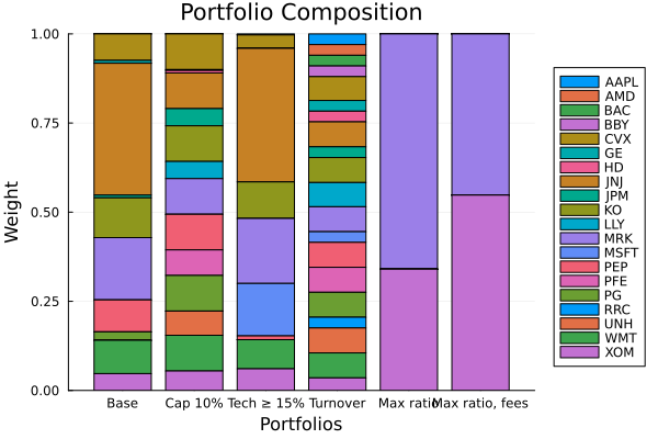
This page was generated using Literate.jl.