The source files can be found in examples/.

Weight drift and held weights: reading a backtest as a fund holds it

A backtest reads a fold in two places, and each place asks a question that has two honest answers.

The first place is the return series. X * w net of fees is the reading the optimiser maximises: it holds the weights fixed and lets the returns arrive. It is the right reading of the decision. It is not the reading of a fund. A fund buys the weights once, and each position then grows at its own return, so what it holds moves away from what it chose. The library calls that movement Weight Drift.

The second place is the weights the next fold starts from. The fold loop threads the previous fold's target weights, so Turnover, TurnoverEstimator, WeightsTracking, TurnoverRiskMeasure and the turnover fee measure the change in the decision. A fund does not trade the change in the decision. It trades the distance from what it holds to what it now wants, and that distance is larger. The library calls the choice between them the Previous-Weights Source.

The two questions are two switches, wd and pws, and they are independent. nothing on either one is the library's original behaviour, so nothing in a caller's existing run moves until that caller sets a field. See docs/adr/0110-the-two-evaluation-switches-are-separate-and-the-library-does-not-bundle-them.md for why the library keeps them apart.

When to reach for this

Reach for wd when the number you report is meant to be the number a fund earned, and the holding period is long enough for the positions to move apart — a quarterly or annual rebalance, a volatile universe, or a book that is not rebalanced between decisions. Reach for pws when something in the optimiser reads previous weights and you want it to bind on the trade rather than on the decision: a turnover cap, a turnover fee, or weights-based tracking. Leave both unset when you are comparing optimisers rather than reporting a fund.

This example runs one walk-forward under both conventions and reads the difference.

The setup: one universe, one optimiser, one walk-forward.
The first switch, on and off, and what it does to the series.
Inside one fold: the weight path, and the weights carried forward.
The second switch, and the turnover cap that means two different things.
The one-off cost and its clock, which is a third switch and orthogonal to both.
What to take away.

using PortfolioOptimisers, CSV, TimeSeries, DataFrames, PrettyTables, Clarabel, Statistics,      StatsPlots# Format for pretty tables.tsfmt = (v, i, j) -> begin    return j == 1 ? Date(v) : vend;pctfmt = (v, i, j) -> begin    return if j == 1        v    else        isa(v, Number) ? "$(round(v * 100, digits = 3)) %" : v    endend;numfmt = (v, i, j) -> begin    return isa(v, Number) ? round(v; sigdigits = 5) : vend;

1. Setting up

Four years of daily data on a small universe. The walk-forward trains on one year and tests on half a year, which is a long enough holding period for the positions to move apart: that is the whole subject of this page, and a fold of a few days would show nothing.

X = TimeArray(CSV.File(joinpath(@__DIR__, "..", "SP500.csv.gz")); timestamp = :Date)[(end - 252 * 4):end]pretty_table(X[(end - 4):end]; formatters = [tsfmt])rd = prices_to_returns(X)N = size(rd.X, 2)slv = Solver(; name = :clarabel, solver = Clarabel.Optimizer,             settings = Dict("verbose" => false),             check_sol = (; allow_local = true, allow_almost = true))mr = MeanRisk(; opt = JuMPOptimiser(; slv = slv))

MeanRisk
  opt ┼ JuMPOptimiser
      │        pe ┼ EmpiricalPrior
      │           │           ce ┼ PortfolioOptimisersCovariance
      │           │              │   ce ┼ Covariance
      │           │              │      │    me ┼ SimpleExpectedReturns
      │           │              │      │       │   w ┴ nothing
      │           │              │      │    ce ┼ GeneralCovariance
      │           │              │      │       │   ce ┼ SimpleCovariance: SimpleCovariance(true)
      │           │              │      │       │    w ┴ nothing
      │           │              │      │   alg ┼ FullMoment()
      │           │              │      │     w ┴ nothing
      │           │              │   mp ┼ MatrixProcessing
      │           │              │      │     pdm ┼ Posdef
      │           │              │      │         │      alg ┼ UnionAll: NearestCorrelationMatrix.Newton
      │           │              │      │         │   kwargs ┴ @NamedTuple{}: NamedTuple()
      │           │              │      │      dn ┼ nothing
      │           │              │      │      dt ┼ nothing
      │           │              │      │     alg ┼ nothing
      │           │              │      │   order ┴ NTuple{4, Symbol}: (:pdm, :dn, :dt, :alg)
      │           │           me ┼ SimpleExpectedReturns
      │           │              │   w ┴ nothing
      │           │      horizon ┼ nothing
      │           │   fill_limit ┴ nothing
      │       slv ┼ Solver
      │           │          name ┼ Symbol: :clarabel
      │           │        solver ┼ UnionAll: Clarabel.MOIwrapper.Optimizer
      │           │      settings ┼ Dict{String, Bool}: Dict{String, Bool}("verbose" => 0)
      │           │     check_sol ┼ @NamedTuple{allow_local::Bool, allow_almost::Bool}: (allow_local = true, allow_almost = true)
      │           │   add_bridges ┴ Bool: true
      │        wb ┼ WeightBounds
      │           │   lb ┼ Float64: 0.0
      │           │   ub ┴ Float64: 1.0
      │       bgt ┼ Float64: 1.0
      │      sbgt ┼ nothing
      │      gbgt ┼ nothing
      │      xbgt ┼ Bool: false
      │        lt ┼ nothing
      │        st ┼ nothing
      │      lcse ┼ nothing
      │       cte ┼ nothing
      │    gcarde ┼ nothing
      │   sgcarde ┼ nothing
      │      smtx ┼ nothing
      │     sgmtx ┼ nothing
      │       slt ┼ nothing
      │       sst ┼ nothing
      │      sglt ┼ nothing
      │      sgst ┼ nothing
      │        tn ┼ nothing
      │      fees ┼ nothing
      │      sets ┼ nothing
      │        tr ┼ nothing
      │       ple ┼ nothing
      │       ret ┼ ArithmeticReturn
      │           │   settings ┼ JuMPReturnsSettings
      │           │            │   scale ┼ Float64: 1.0
      │           │            │      lb ┼ nothing
      │           │            │     rte ┼ Bool: true
      │           │            │     fee ┼ Bool: true
      │           │            │     mic ┴ Bool: true
      │           │        ucs ┼ nothing
      │           │         mu ┴ nothing
      │       sca ┼ SumScalariser()
      │      ccnt ┼ nothing
      │      cobj ┼ nothing
      │        sc ┼ Int64: 1
      │        so ┼ Int64: 1
      │        ss ┼ nothing
      │      card ┼ nothing
      │     scard ┼ nothing
      │       l2c ┼ nothing
      │       lpc ┼ nothing
      │     linfc ┼ nothing
      │        l1 ┼ nothing
      │        l2 ┼ nothing
      │        lp ┼ nothing
      │      linf ┼ nothing
      │       brt ┼ Bool: false
      │     x_src ┼ Symbol: :prior
      │    strict ┴ Bool: false
    r ┼ Variance
      │   settings ┼ RiskMeasureSettings
      │            │   scale ┼ Float64: 1.0
      │            │      ub ┼ nothing
      │            │     rke ┴ Bool: true
      │      sigma ┼ nothing
      │       chol ┼ nothing
      │         rc ┼ nothing
      │        alg ┴ SquaredSOCRiskExpr()
  obj ┼ MinimumRisk()
   wi ┼ nothing
   fb ┴ nothing

Two schemes, identical but for the first switch. SelfFinancingDrift is the one Weight Drift the library ships: every position grows at its own return, the implicit cash position 1 - sum(w) earns nothing, and the weights are quoted against the wealth of the moment, so the held weights and the deflated cash position sum to one at every observation. A fully invested book, which is what MeanRisk builds by default, holds no cash, so its rows keep summing to one; a partly invested book's rows drift with its cash share, and only the sum with the cash holds.

store_weight_path = true asks the drifted scheme to keep the path it computes. A reader who does not ask for it rebuilds the path from the record instead, and the rebuild is bit-identical, so the flag buys time rather than an answer.

wf_target = IndexWalkForward(252, 126)wf_held = IndexWalkForward(252, 126; wd = SelfFinancingDrift(), store_weight_path = true)

IndexWalkForward
         train_size ┼ Int64: 252
          test_size ┼ Int64: 126
        purged_size ┼ Int64: 0
       expand_train ┼ Bool: false
        reduce_test ┼ Bool: false
                 wd ┼ SelfFinancingDrift()
                pws ┼ nothing
                 fa ┼ nothing
  store_weight_path ┼ Bool: true
             strict ┼ Bool: false
                 ff ┴ nothing

2. One walk-forward, two readings

The two runs solve exactly the same optimisation problems. Nothing in the fit changes: the switch is a statement about how a fold's numbers are read, not about how its observations are split or how its weights are chosen.

pred_target = cross_val_predict(mr, rd, wf_target)pred_held = cross_val_predict(mr, rd, wf_held)# The decisions are identical; only the reading of them differs.all(pred_target.res[i].w ≈ pred_held.res[i].w for i in eachindex(pred_target.res))

true

So the two series come from one set of decisions, and every difference between them is the drift.

ret_target = pred_target.mrd.Xret_held = pred_held.mrd.Xsm = LowOrderMoment(; alg = SecondMoment())summary_df = DataFrame(:quantity =>                           ["cumulative return", "mean return", "return volatility",                            "second moment", "worst drawdown"],                       Symbol("target weights") =>                           [prod(1 .+ ret_target) - 1, mean(ret_target), std(ret_target),                            expected_risk(sm, pred_target), minimum(drawdowns(ret_target))],                       Symbol("held weights") =>                           [prod(1 .+ ret_held) - 1, mean(ret_held), std(ret_held),                            expected_risk(sm, pred_held), minimum(drawdowns(ret_held))])pretty_table(summary_df; formatters = [numfmt])

┌───────────────────┬────────────────┬──────────────┐
│          quantity │ target weights │ held weights │
│            String │        Float64 │      Float64 │
├───────────────────┼────────────────┼──────────────┤
│ cumulative return │        0.32338 │      0.29532 │
│       mean return │     0.00045719 │   0.00042588 │
│ return volatility │       0.013163 │     0.012933 │
│     second moment │     0.00017326 │   0.00016726 │
│    worst drawdown │       -0.27454 │     -0.26547 │
└───────────────────┴────────────────┴──────────────┘

The drifted reading is the lower one on every line that measures return, and the lower one on every line that measures risk. Both directions have the same cause. A position that has grown carries a larger share of the book than the optimiser gave it, and a position that has shrunk carries a smaller one, so the drifted book is the book the market built out of the optimiser's choice rather than the book the optimiser chose. On this universe that book earns a little less and moves a little less.

Neither series is the "correct" one. The target series answers what did this rule decide, and the drifted series answers what would a fund holding that decision have earned. The two questions have two answers, and the switch says which one is being asked.

The largest single-day gap between them is the sharpest way to see that the difference is not rounding.

println("largest daily gap between the two readings = $(round(maximum(abs, ret_held .- ret_target) * 100, digits = 4)) %")plot(pred_target.mrd.ts, cumulative_returns(ret_target, true); label = "target weights",     xlabel = "Date", ylabel = "Compound cumulative return", legend = :topleft)plot!(pred_held.mrd.ts, cumulative_returns(ret_held, true); label = "held weights")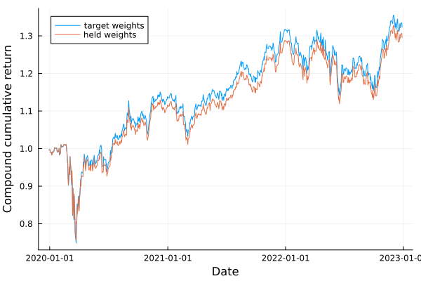

3. Inside one fold: the weight path

A drifted fold carries a Held Weights record, HeldWeightsResult, in the hw field of its PredictionResult. A fold that did not drift carries nothing there, so a consumer that needs a path serves the one and refuses the other by dispatch rather than by a branch.

The record holds four things: the asset returns the fold was scored over, the weight path when the scheme stored it, the weights held after the last observation, and the Weight Drift form that produced them. The last of those is what makes a later rebuild bit-identical.

hw = pred_held.pred[1].hwU = hw.U# The path has one row per observation of the fold and one column per asset.size(U)

(126, 20)

The first row of the path is the target weight vector: the fold starts by holding exactly what it chose. Every row of this fully invested book sums to one, because the drift quotes the positions against the wealth of the moment rather than letting the book inflate.

DataFrame(:row => ["first", "last"], Symbol("sums to") => [sum(U[1, :]), sum(U[end, :])],          Symbol("equals the target") =>              [U[1, :] ≈ pred_held.res[1].w, U[end, :] ≈ pred_held.res[1].w])

2×3 DataFrame

Row	row	sums to	equals the target
	String	Float64	Bool
1	first	1.0	true
2	last	1.0	false

Here is the position that moved furthest over the fold, against the weight the optimiser gave it.

drift = U[end, :] .- U[1, :]j = argmax(abs.(drift))mover_df = DataFrame(:asset => [rd.nx[j]], Symbol("chosen") => [U[1, j]],                     Symbol("held at the end") => [U[end, j]],                     Symbol("drift") => [drift[j]])pretty_table(mover_df; formatters = [pctfmt])

┌────────┬──────────┬─────────────────┬─────────┐
│  asset │   chosen │ held at the end │   drift │
│ String │  Float64 │         Float64 │ Float64 │
├────────┼──────────┼─────────────────┼─────────┤
│    CVX │ 11.588 % │         9.228 % │ -2.36 % │
└────────┴──────────┴─────────────────┴─────────┘

The record's w is not the last row of the path. The last row is what the fund held through the last observation; w is what it holds after that observation has happened, which is one step further on and is what the next fold starts from.

DataFrame(Symbol("largest entry, last path row") => [maximum(U[end, :])],          Symbol("largest entry, carried forward") => [maximum(hw.w)],          Symbol("largest gap between the two") => [maximum(abs, hw.w .- U[end, :])])

1×3 DataFrame

Row	largest entry, last path row	largest entry, carried forward	largest gap between the two
	Float64	Float64	Float64
1	0.241093	0.239703	0.00139017

4. The second switch: which weights the next fold starts from

pws changes nothing at all unless something in the optimiser reads previous weights. Put a turnover cap on the optimiser and it reads them, so the switch decides what the cap is a cap on.

The cap below is 1% per asset per rebalance. Turnover's own w is the starting book of the first fold; factory replaces it fold by fold with whatever the Previous-Weights Source supplies.

cap = 0.01mr_cap = MeanRisk(;                  opt = JuMPOptimiser(; slv = slv,                                      tn = Turnover(; w = fill(1 / N, N), val = cap)))wf_decision = IndexWalkForward(252, 126; wd = SelfFinancingDrift())wf_trade = IndexWalkForward(252, 126; wd = SelfFinancingDrift(), pws = DriftedWeights())pred_decision = cross_val_predict(mr_cap, rd, wf_decision)pred_trade = cross_val_predict(mr_cap, rd, wf_trade)

MultiPeriodPredictionResult
  pred ┼ 6-element Vector{PredictionResult}
       │ PredictionResult ⋯
       │ PredictionResult ⋯
       │ PredictionResult ⋯
       │ PredictionResult ⋯
       │ PredictionResult ⋯
       │ PredictionResult ⋯
   mrd ┼ PredictionReturnsResult
       │     nx ┼ 20-element SubArray{String, 1, Vector{String}, Tuple{Base.Slice{Base.OneTo{Int64}}}, true}
       │      X ┼ 756-element Vector{Float64}
       │     nf ┼ nothing
       │      F ┼ nothing
       │     nb ┼ nothing
       │      B ┼ nothing
       │     ts ┼ 756-element Vector{Date}
       │     iv ┼ nothing
       │   ivpa ┴ nothing
    id ┼ nothing
   opt ┴ nothing

Both of these runs report that they ran sequentially, and neither run in section 2 did. The switch is not the cause: a run goes sequential when the optimiser reads previous weights, which the turnover cap does, and the drift adds no such dependency. That is the reason the library keeps the two switches apart rather than answering both questions with one flag — a caller who wants the fund's reading of the series and nothing else keeps a parallel run.

Two distances can be measured at each rebalance, and they are not the same distance.

The decision change is |w_next - w_prev_target|: how far this fold's answer moved from the last fold's answer.
The executed trade is |w_next - w_prev_held|: how far the fund has to move the book it is actually holding.

function rebalance_distances(pred)    n = length(pred.res)    decision = [maximum(abs, pred.res[i + 1].w .- pred.res[i].w) for i in 1:(n - 1)]    executed = [maximum(abs, pred.res[i + 1].w .- pred.pred[i].hw.w) for i in 1:(n - 1)]    return decision, executedenddec_off, exe_off = rebalance_distances(pred_decision)dec_on, exe_on = rebalance_distances(pred_trade)cap_df = DataFrame(:rebalance => 1:length(dec_off),                   Symbol("source off: decision") => dec_off,                   Symbol("source off: executed") => exe_off,                   Symbol("source on: decision") => dec_on,                   Symbol("source on: executed") => exe_on)pretty_table(cap_df; formatters = [pctfmt])

┌───────────┬──────────────────────┬──────────────────────┬─────────────────────┬─────────────────────┐
│ rebalance │ source off: decision │ source off: executed │ source on: decision │ source on: executed │
│     Int64 │              Float64 │              Float64 │             Float64 │             Float64 │
├───────────┼──────────────────────┼──────────────────────┼─────────────────────┼─────────────────────┤
│         1 │                1.0 % │              2.134 % │             2.867 % │               1.0 % │
│         2 │                1.0 % │              2.531 % │             1.367 % │               1.0 % │
│         3 │                1.0 % │              3.356 % │              2.47 % │               1.0 % │
│         4 │                1.0 % │               2.77 % │             1.685 % │               1.0 % │
│         5 │                1.0 % │              2.452 % │             3.246 % │               1.0 % │
└───────────┴──────────────────────┴──────────────────────┴─────────────────────┴─────────────────────┘

Read the two middle columns first. With the source off, the decision column sits at exactly the cap at every rebalance — the cap is doing its job — and the executed column is two to three times the cap. The constraint was honoured and the fund still traded three times what the caller asked for, because the drift moved the book while the decision stood still.

Now the two right-hand columns. With the source on, it is the executed column that sits at exactly the cap, and the decision column is the one that runs over. That is the same constraint, binding on the quantity a fund actually pays for.

A turnover cap therefore caps the trade only when the Previous-Weights Source says so. The same holds for a turnover fee, for TurnoverRiskMeasure and for WeightsTracking — every consumer that reads a previous weight vector reads whichever one the source supplies.

println("cap per asset per rebalance = $(round(cap * 100, digits = 3)) %")println("largest executed trade, source off = $(round(maximum(exe_off) * 100, digits = 3)) %")println("largest executed trade, source on  = $(round(maximum(exe_on) * 100, digits = 3)) %")

cap per asset per rebalance = 1.0 %
largest executed trade, source off = 3.356 %
largest executed trade, source on  = 1.0 %

5. The one-off cost and its clock

l, s and tn are rates per period. Each of them charges one time on every observation of a return series, at the frequency of the returns. fl and fs are different: they are currency amounts charged one time for the whole holding period, so something must decide where on the series that one charge lands.

That decision is the fa field of Fees and FeesEstimator, and it has two settings. nothing charges the two fixed amounts on the first observation, which is the day the position is opened. AmortisedFees spreads them evenly over the observations instead. It reaches fl and fs alone, and it carries no number: every site that charges a fee knows the observation count it charges over and hands it in.

The two clocks charge the same total. They differ in the drawdown, because one pays the whole cost on the first day and the other pays a share of it on every day.

This is a third switch, and it is orthogonal to the other two: a caller can drift without amortising and amortise without drifting.

w_eq = fill(1 / N, N)fee_first = Fees(; l = 0.0002, fl = 0.001)fee_spread = Fees(; l = 0.0002, fl = 0.001, fa = AmortisedFees())gross = rd.X * w_eqnet_first = calc_net_returns(w_eq, rd.X, fee_first)net_spread = calc_net_returns(w_eq, rd.X, fee_spread)fee_df = DataFrame(:quantity => ["charged in total", "charged on observation 1",                                 "charged on observation 2", "cumulative return"],                   Symbol("on the first observation") =>                       [sum(gross) - sum(net_first), gross[1] - net_first[1],                        gross[2] - net_first[2], prod(1 .+ net_first) - 1],                   Symbol("spread over the series") =>                       [sum(gross) - sum(net_spread), gross[1] - net_spread[1],                        gross[2] - net_spread[2], prod(1 .+ net_spread) - 1])pretty_table(fee_df; formatters = [numfmt])

┌──────────────────────────┬──────────────────────────┬────────────────────────┐
│                 quantity │ on the first observation │ spread over the series │
│                   String │                  Float64 │                Float64 │
├──────────────────────────┼──────────────────────────┼────────────────────────┤
│         charged in total │                   0.2216 │                 0.2216 │
│ charged on observation 1 │                   0.0202 │             0.00021984 │
│ charged on observation 2 │                   0.0002 │             0.00021984 │
│        cumulative return │                  0.87162 │                0.87208 │
└──────────────────────────┴──────────────────────────┴────────────────────────┘

The first row is the same under both clocks, and it is the number calc_total_fees reports: the rate charged on every one of the T observations, plus the fixed amount charged one time.

println("observations = $(size(rd.X, 1))")println("total, by clock  = $(round(calc_total_fees(w_eq, size(rd.X, 1), fee_first), sigdigits = 8)) and $(round(calc_total_fees(w_eq, size(rd.X, 1), fee_spread), sigdigits = 8))")

observations = 1008
total, by clock  = 0.2216 and 0.2216

The fit reads the same clock, and its expected return always spreads

The JuMP model carries the per period terms and the one-off terms in two expressions of its own, and it lays the second onto its net return series on the clock fa names, exactly as the value-level verbs do. Its expected return is a per period number, so the one-off terms always enter it spread over the observation count of the fit, whatever the clock says for a realised series.

6. What to take away

The two switches are independent, and each defaults to the library's original behaviour. A run that sets neither is unchanged.
wd says what a fold's return series means: the decision's reading, or the fund's. It does not change a single weight.
pws says which weights the next fold starts from, and it matters only to the estimators that read previous weights. It changes weights, because it changes what those estimators see.
A turnover cap binds the decision when the source is off, and binds the trade when it is on. The executed trade under a source that is off can be several times the stated cap.
A drifted fold carries a HeldWeightsResult, and a fold that did not drift carries nothing there. The path is rebuilt from the record unless store_weight_path asked for it, and the rebuild is bit-identical.
The weights carried forward are one step beyond the last row of the path, not the last row.
The fee's clock is a third switch, and it reaches the two fixed charges alone. l, s and tn are rates per period and are charged on every observation whatever the clock says. The two clocks charge the same total and give a different drawdown.

This page was generated using Literate.jl.