The source files can be found in examples/.
Feature matrices as a distance source
Every clustering optimiser met so far builds its hierarchy from the returns: a covariance estimate becomes a correlation, a correlation becomes a distance, and the distance becomes a dendrogram. That route can only ever see structure the price history contains.
A FeatureDistance replaces the returns with an assets × features matrix Z. Feature k is any per-asset quantity you can name — a sector membership, a factor loading, a position in the asset network, a trailing characteristic — and two assets are close when their feature rows point the same way. The output is an ordinary distance matrix, so every consumer that takes a distance estimator takes this one: ClustersEstimator, NetworkEstimator, the clustering optimisers, and the phylogeny and centrality constraint families.
The point of the exercise is exogenous structure. A classification, a mandate, a supply chain or a factor model brings in relationships the returns do not contain; feeding the returns graph back in as features is a different and more subtle tool, covered in §4.
Reach for a FeatureDistance when you can name the structure you want the allocation to respect and it is not in the price history — a sector or country taxonomy, a regulatory bucketing, an ESG classification, a factor exposure profile. Reach for it too when you want the hierarchy to stop churning between rebalances: an exogenous classification does not move when the covariance does, which is worth a large turnover reduction (§9). Stay with the ordinary correlation distance when the structure you care about is co-movement.
using PortfolioOptimisers, CSV, TimeSeries, DataFrames, PrettyTables, Clarabel, StatsPlots, GraphRecipes, Statistics, LinearAlgebra, Clusteringresfmt = (v, i, j) -> begin return if j == 1 v else isa(v, AbstractFloat) ? "$(round(v*100, digits=3)) %" : v endend;1. ReturnsResult data and a classification
The same twenty-name S&P 500 slice as the other optimiser examples, plus an illustrative two-level classification. The two levels are nested: every industry belongs to exactly one sector, so agreeing on an industry implies agreeing on a sector.
X = TimeArray(CSV.File(joinpath(@__DIR__, "..", "SP500.csv.gz")); timestamp = :Date)[(end - 252):end]rd = prices_to_returns(X)pr = prior(EmpiricalPrior(), rd)slv = Solver(; name = :clarabel, solver = Clarabel.Optimizer, settings = Dict("verbose" => false), check_sol = (; allow_local = true, allow_almost = true))sector = Dict("AAPL" => "Technology", "AMD" => "Technology", "MSFT" => "Technology", "BAC" => "Financials", "JPM" => "Financials", "CVX" => "Energy", "XOM" => "Energy", "RRC" => "Energy", "GE" => "Industrials", "BBY" => "ConsumerDiscretionary", "HD" => "ConsumerDiscretionary", "KO" => "ConsumerStaples", "PEP" => "ConsumerStaples", "PG" => "ConsumerStaples", "WMT" => "ConsumerStaples", "JNJ" => "HealthCare", "LLY" => "HealthCare", "MRK" => "HealthCare", "PFE" => "HealthCare", "UNH" => "HealthCare")industry = Dict("AAPL" => "ConsumerHardware", "AMD" => "Semiconductors", "MSFT" => "Software", "BAC" => "Banks", "JPM" => "Banks", "CVX" => "IntegratedOil", "XOM" => "IntegratedOil", "RRC" => "ExplorationProduction", "GE" => "Conglomerates", "BBY" => "SpecialtyRetail", "HD" => "SpecialtyRetail", "KO" => "Beverages", "PEP" => "Beverages", "PG" => "HouseholdProducts", "WMT" => "MassMerchants", "JNJ" => "Pharmaceuticals", "LLY" => "Pharmaceuticals", "MRK" => "Pharmaceuticals", "PFE" => "Pharmaceuticals", "UNH" => "ManagedCare")Dict{String, String} with 20 entries:
"MSFT" => "Software"
"JPM" => "Banks"
"MRK" => "Pharmaceuticals"
"UNH" => "ManagedCare"
"PFE" => "Pharmaceuticals"
"BBY" => "SpecialtyRetail"
"BAC" => "Banks"
"PG" => "HouseholdProducts"
"JNJ" => "Pharmaceuticals"
"XOM" => "IntegratedOil"
"LLY" => "Pharmaceuticals"
"AMD" => "Semiconductors"
"CVX" => "IntegratedOil"
"WMT" => "MassMerchants"
"PEP" => "Beverages"
"GE" => "Conglomerates"
"AAPL" => "ConsumerHardware"
"HD" => "SpecialtyRetail"
"KO" => "Beverages"
"RRC" => "ExplorationProduction"The classification travels on a UniverseSets. Every key an asset view has to follow must carry the xkey prefix — "nx_sector", not "sector" — because that prefix is what port_opt_view slices alongside the asset names.
sets = UniverseSets(; xkey = "nx", dict = Dict("nx" => rd.nx, "nx_sector" => [sector[a] for a in rd.nx], "nx_industry" => [industry[a] for a in rd.nx]))taxonomy = ["nx_sector", "nx_industry"]pretty_table(DataFrame("Asset" => rd.nx, "Sector" => [sector[a] for a in rd.nx], "Industry" => [industry[a] for a in rd.nx]); title = "The classification the feature matrix will encode") The classification the feature matrix will encode
┌────────┬───────────────────────┬───────────────────────┐
│ Asset │ Sector │ Industry │
│ String │ String │ String │
├────────┼───────────────────────┼───────────────────────┤
│ AAPL │ Technology │ ConsumerHardware │
│ AMD │ Technology │ Semiconductors │
│ BAC │ Financials │ Banks │
│ BBY │ ConsumerDiscretionary │ SpecialtyRetail │
│ CVX │ Energy │ IntegratedOil │
│ GE │ Industrials │ Conglomerates │
│ HD │ ConsumerDiscretionary │ SpecialtyRetail │
│ JNJ │ HealthCare │ Pharmaceuticals │
│ JPM │ Financials │ Banks │
│ KO │ ConsumerStaples │ Beverages │
│ LLY │ HealthCare │ Pharmaceuticals │
│ MRK │ HealthCare │ Pharmaceuticals │
│ MSFT │ Technology │ Software │
│ PEP │ ConsumerStaples │ Beverages │
│ PFE │ HealthCare │ Pharmaceuticals │
│ PG │ ConsumerStaples │ HouseholdProducts │
│ RRC │ Energy │ ExplorationProduction │
│ UNH │ HealthCare │ ManagedCare │
│ WMT │ ConsumerStaples │ MassMerchants │
│ XOM │ Energy │ IntegratedOil │
└────────┴───────────────────────┴───────────────────────┘2. From a classification to a distance
asset_sets_features stacks one indicator block per key into an assets × features matrix: Z[i, k] == 1 when asset i belongs to group k. asset_sets_feature_names gives the matching column names — take them from there rather than rebuilding the column order by hand, because the block order is the order of taxonomy and the group order inside a block is not something to guess at.
Z = asset_sets_features(taxonomy, sets)nz = asset_sets_feature_names(taxonomy, sets)pretty_table(DataFrame(["Asset" => rd.nx; [nz[k] => Z[:, k] for k in 1:6]...]); title = "The first six feature columns (of $(length(nz)))") The first six feature columns (of 20)
┌────────┬──────────────────────┬──────────────────────┬─────────────────────────────────┬──────────────────┬───────────────────────┬──────────────────────┐
│ Asset │ nx_sector=Technology │ nx_sector=Financials │ nx_sector=ConsumerDiscretionary │ nx_sector=Energy │ nx_sector=Industrials │ nx_sector=HealthCare │
│ String │ Float64 │ Float64 │ Float64 │ Float64 │ Float64 │ Float64 │
├────────┼──────────────────────┼──────────────────────┼─────────────────────────────────┼──────────────────┼───────────────────────┼──────────────────────┤
│ AAPL │ 1.0 │ 0.0 │ 0.0 │ 0.0 │ 0.0 │ 0.0 │
│ AMD │ 1.0 │ 0.0 │ 0.0 │ 0.0 │ 0.0 │ 0.0 │
│ BAC │ 0.0 │ 1.0 │ 0.0 │ 0.0 │ 0.0 │ 0.0 │
│ BBY │ 0.0 │ 0.0 │ 1.0 │ 0.0 │ 0.0 │ 0.0 │
│ CVX │ 0.0 │ 0.0 │ 0.0 │ 1.0 │ 0.0 │ 0.0 │
│ GE │ 0.0 │ 0.0 │ 0.0 │ 0.0 │ 1.0 │ 0.0 │
│ HD │ 0.0 │ 0.0 │ 1.0 │ 0.0 │ 0.0 │ 0.0 │
│ JNJ │ 0.0 │ 0.0 │ 0.0 │ 0.0 │ 0.0 │ 1.0 │
│ JPM │ 0.0 │ 1.0 │ 0.0 │ 0.0 │ 0.0 │ 0.0 │
│ KO │ 0.0 │ 0.0 │ 0.0 │ 0.0 │ 0.0 │ 0.0 │
│ LLY │ 0.0 │ 0.0 │ 0.0 │ 0.0 │ 0.0 │ 1.0 │
│ MRK │ 0.0 │ 0.0 │ 0.0 │ 0.0 │ 0.0 │ 1.0 │
│ MSFT │ 1.0 │ 0.0 │ 0.0 │ 0.0 │ 0.0 │ 0.0 │
│ PEP │ 0.0 │ 0.0 │ 0.0 │ 0.0 │ 0.0 │ 0.0 │
│ PFE │ 0.0 │ 0.0 │ 0.0 │ 0.0 │ 0.0 │ 1.0 │
│ PG │ 0.0 │ 0.0 │ 0.0 │ 0.0 │ 0.0 │ 0.0 │
│ RRC │ 0.0 │ 0.0 │ 0.0 │ 1.0 │ 0.0 │ 0.0 │
│ UNH │ 0.0 │ 0.0 │ 0.0 │ 0.0 │ 0.0 │ 1.0 │
│ WMT │ 0.0 │ 0.0 │ 0.0 │ 0.0 │ 0.0 │ 0.0 │
│ XOM │ 0.0 │ 0.0 │ 0.0 │ 1.0 │ 0.0 │ 0.0 │
└────────┴──────────────────────┴──────────────────────┴─────────────────────────────────┴──────────────────┴───────────────────────┴──────────────────────┘2.1 Why this producer needs no standardisation
asset_sets_matrix builds its groups from the distinct values present, so every key is a partition: each asset lands in exactly one group per key and every row carries exactly L = length(taxonomy) ones. All rows therefore have norm sqrt(L), and the cosine between two assets is exactly
cos(i, j) = shared(i, j) / Lthe count of classification levels they agree on, divided by the number of levels. That makes AngularDist — the default metric — take only L + 1 distinct values, and bounds the distance by 0.5 rather than 1.0 because the cosine can never go negative.
This is the one producer with that property. The others build columns on unrelated scales and have no such guarantee.
D = distance(FeatureDistance(), Z; dims = 1)levels = sort(unique(round.(D; digits = 6)))pretty_table(DataFrame("Quantity" => ["Feature count", "Levels agreed on (L)", "Row norm (every row, = sqrt(L))", "Distinct distances", "The distances themselves"], "Value" => [string(size(Z, 2)), string(length(taxonomy)), string(round(norm(Z[1, :]); digits = 4)), string(length(levels)), string(round.(levels; digits = 4))]); title = "The feature distance this classification produces") The feature distance this classification produces
┌─────────────────────────────────┬────────────────────┐
│ Quantity │ Value │
│ String │ String │
├─────────────────────────────────┼────────────────────┤
│ Feature count │ 20 │
│ Levels agreed on (L) │ 2 │
│ Row norm (every row, = sqrt(L)) │ 1.4142 │
│ Distinct distances │ 3 │
│ The distances themselves │ [0.0, 0.3333, 0.5] │
└─────────────────────────────────┴────────────────────┘Three distances, one per agreement level, up to floating-point noise in acos: 0.0 for two assets in the same industry, 1/3 for two in the same sector but different industries, and 0.5 for two sharing nothing.
2.2 The clustering it produces
The distance goes into an ordinary ClustersEstimator through its de slot. The feature matrix itself is data, not configuration, so it does not live on the estimator — it rides beside the returns and is selected by z_src (§7). Passing it explicitly is the bare form that every optimiser wraps.
onc = OptimalNumberClusters(; alg = 7)cle_cor = ClustersEstimator(; onc = onc)cle_fea = ClustersEstimator(; de = FeatureDistance(), onc = onc)clr_cor = clusterise(cle_cor, pr.X)clr_fea = clusterise(cle_fea, pr.X; Z = Z, z_src = :data)pretty_table(DataFrame("Asset" => rd.nx, "Sector" => [sector[a] for a in rd.nx], "Correlation cut" => cutree(clr_cor.res; k = 4), "Feature cut" => cutree(clr_fea.res; k = 4)); title = "Four-way cuts, correlation against classification") Four-way cuts, correlation against classification
┌────────┬───────────────────────┬─────────────────┬─────────────┐
│ Asset │ Sector │ Correlation cut │ Feature cut │
│ String │ String │ Int64 │ Int64 │
├────────┼───────────────────────┼─────────────────┼─────────────┤
│ AAPL │ Technology │ 1 │ 1 │
│ AMD │ Technology │ 1 │ 1 │
│ BAC │ Financials │ 1 │ 1 │
│ BBY │ ConsumerDiscretionary │ 1 │ 1 │
│ CVX │ Energy │ 2 │ 2 │
│ GE │ Industrials │ 1 │ 1 │
│ HD │ ConsumerDiscretionary │ 1 │ 1 │
│ JNJ │ HealthCare │ 3 │ 3 │
│ JPM │ Financials │ 1 │ 1 │
│ KO │ ConsumerStaples │ 4 │ 4 │
│ LLY │ HealthCare │ 3 │ 3 │
│ MRK │ HealthCare │ 3 │ 3 │
│ MSFT │ Technology │ 1 │ 1 │
│ PEP │ ConsumerStaples │ 4 │ 4 │
│ PFE │ HealthCare │ 3 │ 3 │
│ PG │ ConsumerStaples │ 4 │ 4 │
│ RRC │ Energy │ 2 │ 2 │
│ UNH │ HealthCare │ 3 │ 3 │
│ WMT │ ConsumerStaples │ 4 │ 4 │
│ XOM │ Energy │ 2 │ 2 │
└────────┴───────────────────────┴─────────────────┴─────────────┘On this universe the two agree exactly at four clusters and diverge as the cut goes finer. That is worth reading carefully, because it is the honest result rather than the flattering one: a sector classification and a one-year correlation see the same coarse structure here, and the feature route earns its keep in the fine structure, in the merge order, and — most of all — in what happens when the sample moves (§9).
agreement = DataFrame("k" => 2:10, "Adjusted Rand index" => [round(randindex(cutree(clr_cor.res; k = k), cutree(clr_fea.res; k = k))[1]; digits = 3) for k in 2:10])pretty_table(agreement; title = "How far the two hierarchies agree, cut by cut")plot_dendrogram(clr_fea, rd.nx)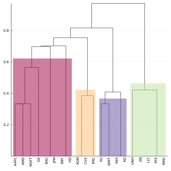
Feeding both hierarchies to HierarchicalRiskParity shows the allocation moving. Note z_src = :data on the HierarchicalOptimiser and the feature matrix carried on a ReturnsResult — that pairing is §7's subject.
rdz = ReturnsResult(; nx = rd.nx, X = rd.X, ts = rd.ts, nz = nz, Z = Z)hrp_cor = optimise(HierarchicalRiskParity(; opt = HierarchicalOptimiser(; pe = pr, cle = cle_cor, slv = slv), r = Variance()), rd)hrp_fea = optimise(HierarchicalRiskParity(; opt = HierarchicalOptimiser(; pe = pr, cle = cle_fea, slv = slv, z_src = :data), r = Variance()), rdz)pretty_table(DataFrame("Asset" => rd.nx, "HRP correlation" => hrp_cor.w, "HRP features" => hrp_fea.w, "Difference" => hrp_fea.w - hrp_cor.w); formatters = [resfmt], title = "Same risk measure, same prior, two hierarchies")plot_stacked_bar_composition([hrp_cor, hrp_fea], rd; xticks = (1:2, ["Correlation", "Features"]))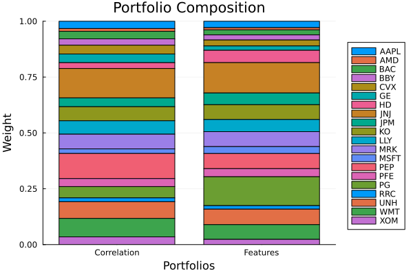
3. The four producers
A feature matrix reaches the library four ways. Three of them are AbstractFeatureMatrixEstimator producers that run inside FeaturePrior and attach Z to the prior result; the fourth is a literal matrix you supply yourself. FeaturePrior delegates every moment to the estimator it wraps and adds nothing but Z, so wrapping never changes the numbers the optimisation is solved on.
3.1 A literal matrix
The simplest producer is no producer at all: hand FeaturePrior the matrix. Use this when the features come from somewhere the library cannot see — a vendor file, a database, your own model.
pr_literal = prior(FeaturePrior(; pe = EmpiricalPrior(), ze = Z), rd)LowOrderPrior
X ┼ 252×20 Matrix{Float64}
o_X ┼ nothing
mu ┼ 20-element Vector{Float64}
sigma ┼ 20×20 Matrix{Float64}
chol ┼ nothing
w ┼ nothing
ens ┼ nothing
kld ┼ nothing
ow ┼ nothing
rr ┼ nothing
fpr ┼ nothing
Z ┴ 20×20 Matrix{Float64}
3.2 AssetSetsFeatures — the exogenous taxonomy
AssetSetsFeatures is §2's classification as a producer, reading its taxonomy from FeaturePrior's sets field. It is the only producer that does not derive Z from the returns, and therefore the only one that brings in structure the price history cannot contain.
pe_taxonomy = FeaturePrior(; pe = EmpiricalPrior(), ze = AssetSetsFeatures(; vals = taxonomy), sets = sets)pr_taxonomy = prior(pe_taxonomy, rd)println("The producer and the public function agree exactly: ", pr_taxonomy.Z == Z)The producer and the public function agree exactly: trueGrading the levels
cos = shared / L weights every level equally, which is rarely what a reader wants — agreeing on an industry is a stronger statement than agreeing on a sector. The vals argument also takes an ordered edge-authoring program of Pairs over a declared feature axis, which writes the weights directly. The axis is declared under sets.zkey, node names are bare, entries apply in order, and the last write wins.
nodes = unique([[sector[a] for a in rd.nx]; [industry[a] for a in rd.nx]])sets_graded = UniverseSets(; xkey = "nx", zkey = "nz", dict = Dict{String, Any}("nx" => rd.nx, "nz" => nodes, "nx_sector" => [sector[a] for a in rd.nx], "nx_industry" => [industry[a] for a in rd.nx]))Z_graded = asset_sets_features(["nx_sector" => 2.0, "nx_industry" => 1.0], sets_graded)D_graded = distance(FeatureDistance(), Z_graded; dims = 1)pretty_table(DataFrame("Pair" => ["AAPL–AMD (same sector, different industry)", "CVX–XOM (same sector, same industry)", "AAPL–KO (nothing shared)"], "Equal levels" => [D[1, 2], D[5, 20], D[1, 10]], "Sector doubled" => [D_graded[1, 2], D_graded[5, 20], D_graded[1, 10]]); formatters = [(v, i, j) -> j == 1 ? v : round(v; digits = 4)], title = "Weighting the coarse level up pulls same-sector pairs together") Weighting the coarse level up pulls same-sector pairs together
┌────────────────────────────────────────────┬──────────────┬────────────────┐
│ Pair │ Equal levels │ Sector doubled │
│ String │ Float64 │ Float64 │
├────────────────────────────────────────────┼──────────────┼────────────────┤
│ AAPL–AMD (same sector, different industry) │ 0.3333 │ 0.2048 │
│ CVX–XOM (same sector, same industry) │ 0.0 │ 0.0 │
│ AAPL–KO (nothing shared) │ 0.5 │ 0.5 │
└────────────────────────────────────────────┴──────────────┴────────────────┘3.3 RegressionFeatures — factor loadings
RegressionFeatures reads the loadings a factor prior has already fitted, so an asset's feature row is its position in the factor coordinate system. This is endogenous — the loadings come from the same returns — but it is a genuinely different reading of them: two assets can load alike and still co-move weakly.
Loadings are signed, which matters for the metric choice in §5.
F = TimeArray(CSV.File(joinpath(@__DIR__, "..", "Factors.csv.gz")); timestamp = :Date)rdf = prices_to_returns(X, F)pr_loadings = prior(FeaturePrior(; pe = FactorPrior(), ze = RegressionFeatures()), rdf)pretty_table(DataFrame(["Asset" => rd.nx; [rdf.nf[k] => pr_loadings.Z[:, k] for k in eachindex(rdf.nf)]...]); formatters = [(v, i, j) -> j == 1 ? v : round(v; digits = 4)], title = "Factor loadings as a feature matrix") Factor loadings as a feature matrix
┌────────┬─────────┬─────────┬─────────┬─────────┬─────────┐
│ Asset │ MTUM │ QUAL │ SIZE │ USMV │ VLUE │
│ String │ Float64 │ Float64 │ Float64 │ Float64 │ Float64 │
├────────┼─────────┼─────────┼─────────┼─────────┼─────────┤
│ AAPL │ 0.0 │ 1.9094 │ -0.7676 │ 0.0 │ 0.0 │
│ AMD │ 0.377 │ 3.0672 │ 0.0 │ -2.1767 │ 0.0 │
│ BAC │ 0.2536 │ 0.0 │ 0.0 │ -0.5916 │ 1.2588 │
│ BBY │ -0.6824 │ 1.2054 │ 0.0 │ 0.0 │ 0.6803 │
│ CVX │ 0.2959 │ 0.0 │ 0.0 │ -0.8437 │ 1.0085 │
│ GE │ 0.0 │ 0.0 │ 0.0 │ 0.0 │ 1.1353 │
│ HD │ -0.3604 │ 0.8314 │ 0.0 │ 0.5918 │ 0.0 │
│ JNJ │ -0.1454 │ 0.0 │ -0.8823 │ 1.3659 │ 0.3754 │
│ JPM │ 0.0 │ -0.6254 │ 0.4967 │ 0.0 │ 1.1515 │
│ KO │ -0.2146 │ -0.487 │ 0.0 │ 1.3327 │ 0.2825 │
│ LLY │ 0.2717 │ 0.0 │ -0.9266 │ 1.6874 │ 0.0 │
│ MRK │ 0.0 │ 0.0 │ -1.1839 │ 1.356 │ 0.5509 │
│ MSFT │ 0.0 │ 2.0455 │ -0.4585 │ 0.0 │ -0.5295 │
│ PEP │ -0.1564 │ 0.0 │ -0.6833 │ 1.5089 │ 0.2629 │
│ PFE │ 0.0 │ 0.0 │ -0.9477 │ 1.3855 │ 0.521 │
│ PG │ -0.2512 │ 0.0 │ -0.7663 │ 1.666 │ 0.3126 │
│ RRC │ 0.0 │ 0.0 │ 0.0 │ 0.0 │ 1.2234 │
│ UNH │ 0.3807 │ -0.9579 │ 0.0 │ 1.7058 │ 0.0 │
│ WMT │ -0.3598 │ 0.0 │ 0.0 │ 1.1136 │ 0.0 │
│ XOM │ 0.4151 │ -0.9477 │ 0.0 │ 0.0 │ 1.2728 │
└────────┴─────────┴─────────┴─────────┴─────────┴─────────┘3.4 PhylogenyFeatures — the returns graph
PhylogenyFeatures turns the asset network into a square assets × assets matrix: feature k reads "how close is this asset to asset k". It is the most endogenous of the four — the graph is filtered out of the correlation — so it does not bring in outside structure. What it does bring is a graded reading of the network that phylogeny_matrix throws away: that routine accumulates a walk count and then clamps it to 0/1, destroying the step count, while this one keeps it.
Its source is always an estimator, never a precomputed result, so the graph is rebuilt on whatever universe the subproblem hands it.
pe_graph = FeaturePrior(; pe = EmpiricalPrior(), ze = PhylogenyFeatures(; pl = NetworkEstimator(; sep = HopCount(; n = 2)), alg = Proximity(; decay = LinearDecay())))pr_graph = prior(pe_graph, rd)pretty_table(DataFrame(["Asset" => rd.nx; [rd.nx[k] => pr_graph.Z[:, k] for k in 1:6]...]); formatters = [(v, i, j) -> j == 1 ? v : round(v; digits = 4)], title = "The first six columns of the graph feature matrix") The first six columns of the graph feature matrix
┌────────┬─────────┬─────────┬─────────┬─────────┬─────────┬─────────┐
│ Asset │ AAPL │ AMD │ BAC │ BBY │ CVX │ GE │
│ String │ Float64 │ Float64 │ Float64 │ Float64 │ Float64 │ Float64 │
├────────┼─────────┼─────────┼─────────┼─────────┼─────────┼─────────┤
│ AAPL │ 3.0 │ 2.0 │ 0.0 │ 0.0 │ 0.0 │ 1.0 │
│ AMD │ 2.0 │ 3.0 │ 0.0 │ 0.0 │ 1.0 │ 2.0 │
│ BAC │ 0.0 │ 0.0 │ 3.0 │ 0.0 │ 0.0 │ 1.0 │
│ BBY │ 0.0 │ 0.0 │ 0.0 │ 3.0 │ 0.0 │ 0.0 │
│ CVX │ 0.0 │ 1.0 │ 0.0 │ 0.0 │ 3.0 │ 2.0 │
│ GE │ 1.0 │ 2.0 │ 1.0 │ 0.0 │ 2.0 │ 3.0 │
│ HD │ 1.0 │ 0.0 │ 0.0 │ 2.0 │ 0.0 │ 0.0 │
│ JNJ │ 1.0 │ 0.0 │ 0.0 │ 0.0 │ 0.0 │ 0.0 │
│ JPM │ 0.0 │ 1.0 │ 2.0 │ 0.0 │ 1.0 │ 2.0 │
│ KO │ 1.0 │ 0.0 │ 0.0 │ 0.0 │ 0.0 │ 0.0 │
│ LLY │ 0.0 │ 0.0 │ 0.0 │ 0.0 │ 0.0 │ 0.0 │
│ MRK │ 0.0 │ 0.0 │ 0.0 │ 0.0 │ 0.0 │ 0.0 │
│ MSFT │ 2.0 │ 1.0 │ 0.0 │ 1.0 │ 0.0 │ 0.0 │
│ PEP │ 2.0 │ 1.0 │ 0.0 │ 0.0 │ 0.0 │ 0.0 │
│ PFE │ 0.0 │ 0.0 │ 0.0 │ 0.0 │ 0.0 │ 0.0 │
│ PG │ 0.0 │ 0.0 │ 0.0 │ 0.0 │ 0.0 │ 0.0 │
│ RRC │ 0.0 │ 0.0 │ 0.0 │ 0.0 │ 1.0 │ 0.0 │
│ UNH │ 1.0 │ 0.0 │ 0.0 │ 0.0 │ 0.0 │ 0.0 │
│ WMT │ 1.0 │ 0.0 │ 0.0 │ 0.0 │ 0.0 │ 0.0 │
│ XOM │ 0.0 │ 0.0 │ 0.0 │ 0.0 │ 2.0 │ 1.0 │
└────────┴─────────┴─────────┴─────────┴─────────┴─────────┴─────────┘Read the diagonal: 3 is the asset itself, 2 a direct neighbour, 1 a two-hop neighbour, 0 unreachable within the budget. §4 explains where those numbers come from — and why they are the one decay setting whose scale depends on the budget.
3.5 The four side by side
producers = DataFrame("Producer" => ["Literal matrix", "AssetSetsFeatures", "RegressionFeatures", "PhylogenyFeatures"], "Feature axis" => ["whatever you supply", "taxonomy groups", "factors / reduced dimensions", "the assets"], "Shape here" => [string(size(Z)), string(size(pr_taxonomy.Z)), string(size(pr_loadings.Z)), string(size(pr_graph.Z))], "Exogenous" => ["depends on the source", "yes", "no", "no"], "Signed" => ["depends on the source", "no", "yes", "no"])pretty_table(producers; title = "The four routes a feature matrix takes") The four routes a feature matrix takes
┌────────────────────┬──────────────────────────────┬────────────┬───────────────────────┬───────────────────────┐
│ Producer │ Feature axis │ Shape here │ Exogenous │ Signed │
│ String │ String │ String │ String │ String │
├────────────────────┼──────────────────────────────┼────────────┼───────────────────────┼───────────────────────┤
│ Literal matrix │ whatever you supply │ (20, 20) │ depends on the source │ depends on the source │
│ AssetSetsFeatures │ taxonomy groups │ (20, 20) │ yes │ no │
│ RegressionFeatures │ factors / reduced dimensions │ (20, 5) │ no │ yes │
│ PhylogenyFeatures │ the assets │ (20, 20) │ no │ no │
└────────────────────┴──────────────────────────────┴────────────┴───────────────────────┴───────────────────────┘4. Two knobs on the graph producer, and neither implies the other
PhylogenyFeatures is driven by two settings that live on two different objects:
sepon theNetworkEstimatordecides which pairs are related — how far apart two assets may sit and still score above zero.HopCountcounts edges with a budget ofnof them;PathLengthsums distances along the shortest path with a budgetdmaxin those units.decayonProximitydecides how strongly a related pair scores as separation grows.
Setting one does not imply the other, and getting that wrong produces no error at all. The confusion is easy to fall into because the default pairing hides it: under LinearDecay with HopCount, the budget is the top of the scale, so changing sep appears to change the fall-off too. Under any other decay the two separate cleanly.
separations = ["HopCount(; n = 2)" => HopCount(; n = 2), "PathLength(; dmax = 1.0)" => PathLength(; dmax = 1.0)]decays = ["LinearDecay()" => LinearDecay(), "ExponentialDecay()" => ExponentialDecay(), "ReciprocalDecay()" => ReciprocalDecay(), "NoDecay()" => NoDecay()]function graph_features(sep, decay) ze = PhylogenyFeatures(; pl = NetworkEstimator(; sep = sep), alg = Proximity(; decay = decay)) return prior(FeaturePrior(; pe = EmpiricalPrior(), ze = ze), rd).Zendsweep = DataFrame()for (sname, sep) in separations, (dname, decay) in decays Zg = graph_features(sep, decay) off = [Zg[i, j] for i in axes(Zg, 1) for j in axes(Zg, 2) if i != j] Dg = distance(FeatureDistance(), Zg; dims = 1) clg = clusterise(cle_fea, pr.X; Z = Zg, z_src = :data) append!(sweep, DataFrame("Separation" => sname, "Decay" => dname, "Self score" => Zg[1, 1], "Largest off-diagonal" => maximum(off), "Related pairs" => count(!iszero, off), "ARI vs correlation" => randindex(cutree(clr_cor.res; k = 4), cutree(clg.res; k = 4))[1]))endpretty_table(sweep; formatters = [(v, i, j) -> isa(v, AbstractFloat) ? round(v; digits = 4) : v], title = "Four decays crossed against two separations") Four decays crossed against two separations
┌──────────────────────────┬────────────────────┬────────────┬──────────────────────┬───────────────┬────────────────────┐
│ Separation │ Decay │ Self score │ Largest off-diagonal │ Related pairs │ ARI vs correlation │
│ String │ String │ Float64 │ Float64 │ Int64 │ Float64 │
├──────────────────────────┼────────────────────┼────────────┼──────────────────────┼───────────────┼────────────────────┤
│ HopCount(; n = 2) │ LinearDecay() │ 3.0 │ 2.0 │ 96 │ 0.4762 │
│ HopCount(; n = 2) │ ExponentialDecay() │ 1.0 │ 0.3679 │ 96 │ 0.4762 │
│ HopCount(; n = 2) │ ReciprocalDecay() │ 1.0 │ 0.5 │ 96 │ 0.5053 │
│ HopCount(; n = 2) │ NoDecay() │ 1.0 │ 1.0 │ 96 │ 0.2842 │
│ PathLength(; dmax = 1.0) │ LinearDecay() │ 2.0 │ 1.7747 │ 94 │ 0.4471 │
│ PathLength(; dmax = 1.0) │ ExponentialDecay() │ 1.0 │ 0.7983 │ 94 │ 0.5274 │
│ PathLength(; dmax = 1.0) │ ReciprocalDecay() │ 1.0 │ 0.8161 │ 94 │ 0.4471 │
│ PathLength(; dmax = 1.0) │ NoDecay() │ 1.0 │ 1.0 │ 94 │ 0.2842 │
└──────────────────────────┴────────────────────┴────────────┴──────────────────────┴───────────────┴────────────────────┘Read the table down the columns rather than across the rows:
Related pairsmoves with the separation and never with the decay. Which pairs are related issep's question alone.Self scoreis1.0for every decay exceptLinearDecay, where it is the budget plus one —3underHopCount(; n = 2),2underPathLength(; dmax = 1.0). The other three pinf(0) = 1and set the fall-off from their own parameter, independently of how far the budget looks. That is the whole of the coincidence: under the default pairing the budget doubles as the scale, and under every other it does not.ARI vs correlationmoves with both. The decay is not cosmetic — it changes the distance and the clusters that come out of it.NoDecayis not "no truncation". The budget still cuts, so it gives1inside and0outside: a neighbourhood indicator, not a matrix of ones. It is also the row where the two separations agree exactly, because an indicator can only see the support.
plot(1:size(sweep, 1), sweep[!, "ARI vs correlation"]; marker = :circle, legend = false, xticks = (1:size(sweep, 1), [string(first(split(r.Separation, "(")), " / ", first(split(r.Decay, "("))) for r in eachrow(sweep)]), xrotation = 45, ylabel = "Adjusted Rand index against the correlation cut", title = "Both knobs move the clustering")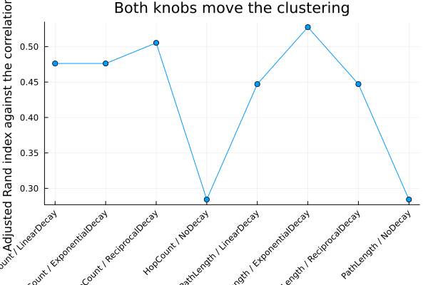
PathLength() with no dmax means the whole connected component. On this path that is a sensible choice — the budget only sets where the fall-off reaches zero, and the decay still grades everything inside it. On the constraint path the identical setting selects instead of shaping, so it declares every reachable pair related and forbids all pairwise co-movement, optimising successfully into a one-asset portfolio. See Phylogeny and centrality constraints §2.2 for that end of it. The bare default also makes the scale of Z depend on the sample — §8.2.
5. Metrics, and the similarity slot
FeatureDistance's metric field takes any Distances.SemiMetric, including one you define. The default is AngularDist, which is the arc-cosine of the cosine similarity scaled to [0, 1] and delegates to Distances' BLAS gemm path.
The choice is not free. Metrics differ in what they are defined on, and one of them fails silently on input outside its domain, which is why the library checks the domain rather than trusting it.
metrics = ["AngularDist()" => AngularDist(), "Distances.CosineDist()" => PortfolioOptimisers.Distances.CosineDist(), "Distances.Jaccard()" => PortfolioOptimisers.Distances.Jaccard()]metric_rows = DataFrame()for (mname, metric) in metrics de = FeatureDistance(; metric = metric) Dm = distance(de, Z; dims = 1) append!(metric_rows, DataFrame("Metric" => mname, "Default similarity" => strip(string(de.sim)), "Maximum distance" => round(maximum(Dm); digits = 4), "Distinct values" => length(unique(round.(Dm; digits = 6)))))endpretty_table(metric_rows; title = "Three metrics on the same classification matrix") Three metrics on the same classification matrix
┌────────────────────────┬────────────────────────┬──────────────────┬─────────────────┐
│ Metric │ Default similarity │ Maximum distance │ Distinct values │
│ String │ SubString{String} │ Float64 │ Int64 │
├────────────────────────┼────────────────────────┼──────────────────┼─────────────────┤
│ AngularDist() │ AngularSimilarity() │ 0.5 │ 3 │
│ Distances.CosineDist() │ ComplementSimilarity() │ 1.0 │ 3 │
│ Distances.Jaccard() │ ComplementSimilarity() │ 1.0 │ 3 │
└────────────────────────┴────────────────────────┴──────────────────┴─────────────────┘On a partition matrix all three order the pairs identically — only the scale differs, and AngularDist stops at 0.5 because a non-negative matrix admits no negative cosine. They part company as soon as the matrix is signed:
signed_metric = try distance(FeatureDistance(; metric = PortfolioOptimisers.Distances.Jaccard()), pr_loadings.Z; dims = 1) "no error"catch err sprint(showerror, err)endprintln(signed_metric)DomainError with all(x -> 0 <= x, Z) must hold. Got
all(x -> 0 <= x, Z) => false:Distances.Jaccard is the Ruzicka form, defined only on non-negative reals, and on signed input it returns values up to 2 with no complaint at all — straight into a clustering routine. The domain check turns that silence into the error above; it covers Distances.BrayCurtis and Distances.ChiSqDist too. Signed feature matrices — factor loadings above all — want AngularDist or Distances.CosineDist.
The sim slot
Clustering consumers call cor_and_dist, not distance, so a feature distance owes a similarity matrix as well. sim supplies it, defaulted from the metric by default_similarity: AngularDist gets AngularSimilarity, which recovers the cosine exactly as cos(πD), and everything else gets ComplementSimilarity's 1 - D. Set it explicitly to override.
clr_pair = cor_and_dist(FeatureDistance(), nothing, pr.X; Z = Z, z_src = :data)println("S and D share provenance: ", size(clr_pair[1]) == size(clr_pair[2]))S and D share provenance: true6. Both shapes: static and time-varying
A feature matrix is either static (assets × features) or time-varying (observations × assets × features, observations leading). The shape is read from ndims, with no wrapper type. A time-varying matrix has to become one distance matrix somehow, and the alg field says how — an open family with four members.
Here the features are two trailing characteristics that genuinely move: annualised realised volatility over twenty-one days, and cumulative return over sixty-three.
T, N = size(rd.X)Ztv = zeros(T, N, 2)for t in 1:T lo_vol = max(1, t - 20) lo_mom = max(1, t - 62) for i in 1:N Ztv[t, i, 1] = std(view(rd.X, lo_vol:t, i)) * sqrt(252) Ztv[t, i, 2] = sum(view(rd.X, lo_mom:t, i)) endendZtv[1, :, 1] .= Ztv[2, :, 1]collapses = ["LastObservation()" => LastObservation(), "AggregateFeatures()" => AggregateFeatures(), "AggregateDistances()" => AggregateDistances(), "StackObservations()" => StackObservations()]collapse_rows = DataFrame()for (cname, alg) in collapses Dc = distance(FeatureDistance(; alg = alg), Ztv; dims = 1) D1 = distance(FeatureDistance(; alg = alg), reshape(Ztv[end, :, :], 1, N, 2); dims = 1) append!(collapse_rows, DataFrame("Collapse" => cname, "Mean distance" => round(mean(Dc); digits = 4), "Maximum distance" => round(maximum(Dc); digits = 4), "Mean at T = 1" => round(mean(D1); digits = 6)))endpretty_table(collapse_rows; title = "Four collapse rules on one $(T)×$(N)×2 feature matrix") Four collapse rules on one 252×20×2 feature matrix
┌──────────────────────┬───────────────┬──────────────────┬───────────────┐
│ Collapse │ Mean distance │ Maximum distance │ Mean at T = 1 │
│ String │ Float64 │ Float64 │ Float64 │
├──────────────────────┼───────────────┼──────────────────┼───────────────┤
│ LastObservation() │ 0.1243 │ 0.4684 │ 0.12428 │
│ AggregateFeatures() │ 0.0739 │ 0.2265 │ 0.12428 │
│ AggregateDistances() │ 0.1163 │ 0.2197 │ 0.12428 │
│ StackObservations() │ 0.1613 │ 0.2731 │ 0.12428 │
└──────────────────────┴───────────────┴──────────────────┴───────────────┘The four rules give four different answers, and they are different in kind:
LastObservation(the default) takes the most recent slice and ignores the rest.AggregateFeaturesaverages the features first, then measures once.AggregateDistancesmeasures each period, then averages the distance matrices. It refusesMedianCollapseat construction, because a convex combination of metrics is a metric while a median of distance matrices is not.StackObservationsconcatenates every period into one long coordinate vector. It is the most scale-exposed of the four, since a period with large magnitudes dominates.
The last column is the degeneracy that shows they are the same idea: at one observation all four agree exactly. A static matrix never reads alg at all — it is inert there, not an error, because z_src legitimately switches between static and time-varying sources.
Both aggregating rules take observation weights on a w field, so an exponential decay or an entropy-pooling posterior reaches the collapse.
6.1 A producer can emit this shape, and it tracks a fold for free
The matrix above was built by hand and carried on the returns. The derived carrier takes the same shape, and a producer is the way to put it there. Nothing in the library ships one — every shipped producer returns assets × features — but the interface has no shape constraint, and a producer is handed the subproblem's own returns, so a time-varying Z comes out with exactly the rows the fit was given.
That is worth stating plainly because it is the answer to the failure in §8.1: a producer never has to be resliced, because it recomputes. A rolling-dispersion producer is about ten lines —
struct TrailingDispersionFeatures <: PortfolioOptimisers.AbstractFeatureMatrixEstimator windows::Vector{Int}endfunction PortfolioOptimisers.feature_matrix(ze::TrailingDispersionFeatures, ::PortfolioOptimisers.AbstractPriorResult, X::PortfolioOptimisers.MatNum, args...; kwargs...) T, N = size(X) Z = zeros(T, N, length(ze.windows)) for (k, w) in pairs(ze.windows), t in 1:T, i in 1:N Z[t, i, k] = std(view(X, max(1, t - w + 1):t, i)) end Z[1, :, :] .= Z[2, :, :] return Zend— and fitting it on the full sample gives (252, 20, 2) while fitting it on the first hundred rows gives (100, 20, 2), with no clock, no indices and no plumbing. Cross-validation cannot take precomputed quantities in any case, so anything a fold reads has to be computed per fold, and a producer is what "computed per fold" means here.
plot([distance(FeatureDistance(; alg = alg), Ztv; dims = 1)[1, :] for (_, alg) in collapses]; label = reshape([c for (c, _) in collapses], 1, :), marker = :circle, xticks = (1:N, rd.nx), xrotation = 90, ylabel = "Distance from AAPL", title = "The collapse rule is a modelling choice, not a detail")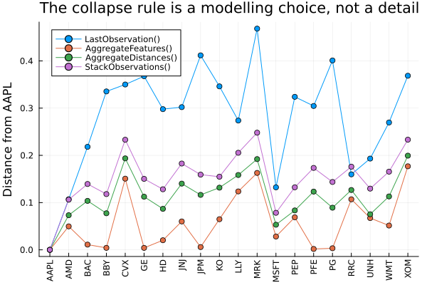
7. Two carriers, one selector
A feature matrix reaches distance from one of two places, and z_src on the optimiser picks which:
z_src = :datareadsReturnsResult'sZ— the matrix you supplied. This is the default, because an explicitly supplied matrix outranks a derived one. It is the opposite default tox_src, deliberately.z_src = :priorreads the prior result'sZ— the matrix a producer derived.
Provenance is strict: a producer only ever populates the prior carrier, and prior(pe, rd) always drops rd.Z. The two carriers therefore never hold two copies of one matrix, and z_src never picks between two spellings of the same thing.
7.1 Outside a fold the two routes agree
Given the same classification, the two routes are indistinguishable.
hrp_data = optimise(HierarchicalRiskParity(; opt = HierarchicalOptimiser(; pe = pr, cle = cle_fea, slv = slv, z_src = :data), r = Variance()), rdz)hrp_prior = optimise(HierarchicalRiskParity(; opt = HierarchicalOptimiser(; pe = pe_taxonomy, cle = cle_fea, slv = slv, z_src = :prior), r = Variance()), rd)println("Largest weight difference between the two carriers: ", round(maximum(abs, hrp_data.w - hrp_prior.w); digits = 12))Largest weight difference between the two carriers: 0.07.2 Inside a fold they are two different semantics
The equality above is a property of the whole universe, not of the two selectors. Under a meta-optimiser or a cross-validation fold:
:dataslices. The carried matrix is subselected to the subproblem's assets. Its columns still describe the classification of the full universe.:priorrefits. The producer runs again inside the subproblem's ownpriorcall and recomputesZfrom the subproblem's returns and its slicedUniverseSets.
For an exogenous taxonomy the two coincide, because slicing a partition and re-deriving it give the same thing. For a returns-derived producer they do not: PhylogenyFeatures rebuilds the graph on the cluster it is handed, so its features describe that cluster's topology, while a carried copy of the full-universe graph describes the universe's.
7.3 The one shape where slicing and measuring do not commute
The rule that decides this is features_are_assets, and it compares names, not axis lengths: when nz == nx the feature axis is the asset axis, so an asset view slices it too. That makes a square, asset-keyed matrix the one shape where measuring a subproblem is not the same as reading a subproblem out of the universe's distance matrix.
Z_square = phylogeny_features(Proximity(; decay = LinearDecay()), NetworkEstimator(; sep = HopCount(; n = 2)), pr.X)rd_square = ReturnsResult(; nx = rd.nx, X = rd.X, ts = rd.ts, nz = rd.nx, Z = Z_square)subset = [1, 2, 3, 5, 8, 10, 13, 17]view_square = PortfolioOptimisers.port_opt_view(rd_square, subset)view_rect = PortfolioOptimisers.port_opt_view(rdz, subset)commute = DataFrame("Feature axis" => ["The assets (square)", "Taxonomy groups (rectangular)"], "Shape of the view" => [string(size(view_square.Z)), string(size(view_rect.Z))], "Largest disagreement" => [maximum(abs, distance(FeatureDistance(), Z_square; dims = 1)[subset, subset] - distance(FeatureDistance(), view_square.Z; dims = 1)), maximum(abs, distance(FeatureDistance(), Z; dims = 1)[subset, subset] - distance(FeatureDistance(), view_rect.Z; dims = 1))])pretty_table(commute; formatters = [(v, i, j) -> isa(v, AbstractFloat) ? round(v; digits = 4) : v], title = "Measuring the subproblem against measuring the universe") Measuring the subproblem against measuring the universe
┌───────────────────────────────┬───────────────────┬──────────────────────┐
│ Feature axis │ Shape of the view │ Largest disagreement │
│ String │ String │ Float64 │
├───────────────────────────────┼───────────────────┼──────────────────────┤
│ The assets (square) │ (8, 8) │ 0.0768 │
│ Taxonomy groups (rectangular) │ (8, 20) │ 0.0 │
└───────────────────────────────┴───────────────────┴──────────────────────┘The rectangular case agrees to the last bit: its columns are the same twenty groups whichever assets you keep, so slicing rows and measuring commute. The square case does not, and the gap is not noise — it is the difference between "how close are these two assets within this cluster" and "how close are they in the whole universe". Neither reading is wrong; they are different questions, and the shape of Z is what chooses between them.
The prior carrier has no squareness vocabulary at all, and that is deliberate: a derived Z is never cut down its feature axis, because a producer refits on whatever universe it is given rather than slicing a description of a larger one.
7.4 A meta-optimiser's outer problem
A meta-optimiser's outer problem is defined over synthetic assets — sub-portfolios, clusters, predictions — which have no rows in any feature matrix. The outer problem is nevertheless feature-capable: the inner universe's Z is collapsed onto the synthetic assets by the inner weights, so an outer FeatureDistance measures the sub-portfolios' features rather than failing.
nco = NestedClustered(; pe = pr, cle = cle_fea, z_src = :data, opti = HierarchicalRiskParity(; opt = HierarchicalOptimiser(; pe = pr, cle = cle_cor, slv = slv), r = Variance()), opto = HierarchicalRiskParity(; opt = HierarchicalOptimiser(; cle = cle_fea, slv = slv, z_src = :data), r = Variance()))res_nco = optimise(nco, rdz)println("Outer problem solved on collapsed features: ", isa(res_nco.retcode, OptimisationSuccess))Outer problem solved on collapsed features: trueA rectangular matrix keeps its own feature axis through that collapse — a cluster's row reads "this cluster's weighted-average membership of each group". A square, asset-keyed one is contracted on both axes at once, so it stays square on the synthetic universe.
8. What changes once cross-validation is switched on
Two behaviours are invisible until the sample starts moving, and both surface as surprises.
8.1 A time-varying literal cannot survive an observation fold
The observation counts always match when you build the matrix — the fold is what breaks them, and it breaks them on one carrier only.
A literal ze sits on the estimator, and the view layer hands an estimator asset indices and nothing else. So port_opt_view cuts the literal's asset axis and leaves its observation axis untouched, while the returns lose every row outside the fold. A Z carried on the ReturnsResult is data, and its view takes observations as well as assets, so it follows.
Ztv_wide = zeros(2 * T, N, 2)Ztv_wide[1:T, :, :] .= ZtvZtv_wide[(T + 1):end, :, :] .= Ztvview_estimator = PortfolioOptimisers.port_opt_view(FeaturePrior(; pe = EmpiricalPrior(), ze = Ztv_wide), [1, 2, 3])view_carried = PortfolioOptimisers.port_opt_view(ReturnsResult(; nx = rd.nx, X = rd.X, ts = rd.ts, nz = ["volatility", "momentum"], Z = Ztv), 1:100, [1, 2, 3])pretty_table(DataFrame("Carrier" => ["Estimator-held literal `ze`", "ReturnsResult `Z`"], "Before the view" => [string(size(Ztv_wide)), string(size(Ztv))], "After the view" => [string(size(view_estimator.ze)), string(size(view_carried.Z))], "Observation axis" => ["untouched", "sliced"]); title = "Only one of the two carriers can follow an observation fold") Only one of the two carriers can follow an observation fold
┌─────────────────────────────┬─────────────────┬────────────────┬──────────────────┐
│ Carrier │ Before the view │ After the view │ Observation axis │
│ String │ String │ String │ String │
├─────────────────────────────┼─────────────────┼────────────────┼──────────────────┤
│ Estimator-held literal `ze` │ (504, 20, 2) │ (504, 3, 2) │ untouched │
│ ReturnsResult `Z` │ (252, 20, 2) │ (100, 3, 2) │ sliced │
└─────────────────────────────┴─────────────────┴────────────────┴──────────────────┘The consequence is that a fit whose observation count has changed cannot line up, and it says so rather than guessing:
fold_error = try prior(FeaturePrior(; pe = EmpiricalPrior(), ze = Ztv), rd.X[1:100, :]) "no error"catch err sprint(showerror, err)endprintln(fold_error)DimensionMismatch: a literal time-varying feature matrix on `FeaturePrior.ze` cannot follow an observation fold. The view layer hands an estimator asset indices only, so its observation axis stays at its original length while the returns are cut to the fold, and nothing can recover which rows to keep. Got size(ze, 1) = 252 and 100 observations. Three ways forward, best first:
1. Compute the features with a producer (an `AbstractFeatureMatrixEstimator` with a `feature_matrix` method). A producer is handed the fold's own `X`, so a time-varying `Z` tracks the fold with no extra plumbing — the derived carrier supports the shape, nothing shipped emits it yet.
2. Carry the matrix on the `ReturnsResult` as `Z` and read it with `z_src = :data`. There it is data, so the fold slices its observation axis alongside `X`.
3. Pass a static assets × features matrix, which has no observation axis to fall out of step.The error is loud and names the two counts, which is the whole point — the alternative is a feature matrix silently describing the wrong periods. Construction succeeds, an asset view succeeds, and a fit on the full sample succeeds: only a changed observation count fails, which is why cross-validation is where this surfaces and nothing before it does.
The message names three ways forward, best first:
- Compute the features with a producer (§6.1). It is handed the fold's own returns, so a time-varying
Ztracks the fold with nothing to reslice. This is the answer for most people who hit the error, and the only one that also works on the derived carrier. - Carry the matrix on the
ReturnsResultand read it withz_src = :data. There it is data, so the fold slices its observation axis alongsideX— the second row of the table above. - Pass a static
assets × featuresmatrix, which has no observation axis to fall out of step.
Note what the failure is not: it is not the derived carrier refusing a time-varying shape. It accepts one, and a producer emits one. The refusal is narrower — a matrix that was computed in advance cannot be recomputed for a subproblem, and cross-validation cannot take precomputed quantities in any case.
Slicing the observation axis with asset indices is what an automatically generated view would have done here, and it would have been finite, plausible and wrong. The view is hand-written to refuse that trade.
8.2 A bare PathLength() makes the scale of Z sample-dependent
PathLength with no dmax resolves its budget to the graph's observed diameter. Under LinearDecay the top of the scale is the budget plus one, so a diameter that moves between folds moves the whole matrix with it. Rolling a one-year window forward a quarter at a time over five years:
Xb = TimeArray(CSV.File(joinpath(@__DIR__, "..", "SP500.csv.gz")); timestamp = :Date)[(end - 1260):end]rdb = prices_to_returns(Xb)windows = [(i, i + 251) for i in 1:63:(size(rdb.X, 1) - 251)]function window_row(lo, hi) Xw = prior(EmpiricalPrior(), rdb.X[lo:hi, :]).X seps = separation_matrix(PathLength(), NetworkEstimator(), Xw) Zbare = phylogeny_features(Proximity(; decay = LinearDecay()), NetworkEstimator(; sep = PathLength()), Xw) Zfixed = phylogeny_features(Proximity(; decay = LinearDecay()), NetworkEstimator(; sep = PathLength(; dmax = 1.5)), Xw) return (; Window = "$(lo)–$(hi)", var"Observed diameter" = maximum(filter(isfinite, seps)), var"Self score, bare" = Zbare[1, 1], var"Self score, dmax = 1.5" = Zfixed[1, 1])enddiameters = DataFrame([window_row(lo, hi) for (lo, hi) in windows])pretty_table(diameters; formatters = [(v, i, j) -> isa(v, AbstractFloat) ? round(v; digits = 4) : v], title = "The bare budget follows the sample; a stated one does not")plot(1:length(windows), diameters[!, "Self score, bare"]; marker = :circle, label = "PathLength()", xlabel = "Rolling window", ylabel = "Top of the Z scale", title = "A data-dependent budget moves the whole feature matrix")plot!(1:length(windows), diameters[!, "Self score, dmax = 1.5"]; marker = :square, label = "PathLength(; dmax = 1.5)")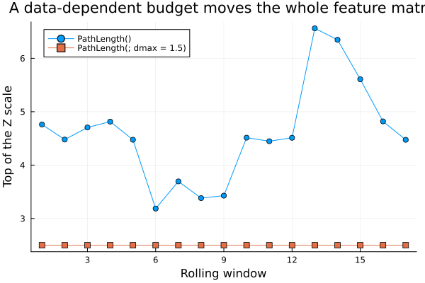
The diameter roughly doubles across these windows and the scale follows it exactly. What makes that worse than it sounds is how it moves. The difference between a bare budget and a stated one is a constant added to every in-budget entry, not a factor multiplying them:
Xw1 = prior(EmpiricalPrior(), rdb.X[1:252, :]).XZ_bare = phylogeny_features(Proximity(; decay = LinearDecay()), NetworkEstimator(; sep = PathLength()), Xw1)Z_fixed = phylogeny_features(Proximity(; decay = LinearDecay()), NetworkEstimator(; sep = PathLength(; dmax = 3.0)), Xw1)shared = (Z_bare .!= 0) .&& (Z_fixed .!= 0)D_bare = distance(FeatureDistance(), Z_bare; dims = 1)D_scaled = distance(FeatureDistance(), 7.3 .* Z_bare; dims = 1)Z_shifted = copy(Z_bare)Z_shifted[Z_bare .!= 0] .+= 1.0D_shifted = distance(FeatureDistance(), Z_shifted; dims = 1)pretty_table(DataFrame("Quantity" => ["Distinct differences on the shared support", "The difference itself", "Distance change from rescaling Z by 7.3", "Distance change from adding 1.0 on the support"], "Value" => [string(length(unique(round.(Z_bare[shared] - Z_fixed[shared]; digits = 8)))), string(round(first(unique(round.(Z_bare[shared] - Z_fixed[shared]; digits = 8))); digits = 6)), string(round(maximum(abs, D_scaled - D_bare); digits = 12)), string(round(maximum(abs, D_shifted - D_bare); digits = 4))]); title = "A shift is not a rescale, and only one of them is invisible") A shift is not a rescale, and only one of them is invisible
┌────────────────────────────────────────────────┬──────────┐
│ Quantity │ Value │
│ String │ String │
├────────────────────────────────────────────────┼──────────┤
│ Distinct differences on the shared support │ 1 │
│ The difference itself │ 0.761185 │
│ Distance change from rescaling Z by 7.3 │ 0.0 │
│ Distance change from adding 1.0 on the support │ 0.0603 │
└────────────────────────────────────────────────┴──────────┘AngularDist is invariant to rescaling an asset's whole row — that is why the third row is zero to machine precision — but a shift changes the direction the row points, and the fourth row is the proof. So a moving diameter is not absorbed by the metric's invariance: it reshapes the distance fold by fold.
Two ways out, and both are one keyword:
- State a numeric
dmax, which pins the budget and the scale across every fold. - Use a decay that pins
f(0) = 1—ExponentialDecay,ReciprocalDecayorNoDecay— which never had the exposure in the first place.
9. A walk-forward backtest
The sharpest argument for an exogenous feature matrix is what it does to stability. A correlation hierarchy is refitted from scratch every fold and moves whenever the covariance does; a classification does not move at all. Walking forward over five years with one-year training windows and quarterly rebalances:
Z_bt = asset_sets_features(taxonomy, UniverseSets(; xkey = "nx", dict = Dict("nx" => rdb.nx, "nx_sector" => [sector[a] for a in rdb.nx], "nx_industry" => [industry[a] for a in rdb.nx])))rdbz = ReturnsResult(; nx = rdb.nx, X = rdb.X, ts = rdb.ts, nz = nz, Z = Z_bt)walk = IndexWalkForward(252, 63)bt_cor = cross_val_predict(HierarchicalRiskParity(; opt = HierarchicalOptimiser(; pe = EmpiricalPrior(), cle = ClustersEstimator(), slv = slv), r = Variance()), rdb, walk)bt_fea = cross_val_predict(HierarchicalRiskParity(; opt = HierarchicalOptimiser(; pe = EmpiricalPrior(), cle = ClustersEstimator(; de = FeatureDistance()), slv = slv, z_src = :data), r = Variance()), rdbz, walk)function backtest_row(name, p) r = p.mrd.X turn = mean(abs, reduce(vcat, [p.pred[i + 1].res.w - p.pred[i].res.w for i in 1:(length(p.pred) - 1)])) return (; Hierarchy = name, var"Annual return" = mean(r) * 252, var"Annual volatility" = std(r) * sqrt(252), var"Sharpe ratio" = mean(r) / std(r) * sqrt(252), var"Maximum drawdown" = expected_risk(MaximumDrawdown(), p), var"Mean weight change" = turn)endpretty_table(DataFrame([backtest_row("Correlation", bt_cor), backtest_row("Classification", bt_fea)]); formatters = [(v, i, j) -> isa(v, AbstractFloat) ? round(v; digits = 4) : v], title = "Out-of-sample, $(length(bt_cor.pred)) quarterly rebalances") Out-of-sample, 16 quarterly rebalances
┌────────────────┬───────────────┬───────────────────┬──────────────┬──────────────────┬────────────────────┐
│ Hierarchy │ Annual return │ Annual volatility │ Sharpe ratio │ Maximum drawdown │ Mean weight change │
│ String │ Float64 │ Float64 │ Float64 │ Float64 │ Float64 │
├────────────────┼───────────────┼───────────────────┼──────────────┼──────────────────┼────────────────────┤
│ Correlation │ 0.197 │ 0.1956 │ 1.0071 │ 0.3085 │ 0.0124 │
│ Classification │ 0.1977 │ 0.1956 │ 1.0108 │ 0.2915 │ 0.0054 │
└────────────────┴───────────────┴───────────────────┴──────────────┴──────────────────┴────────────────────┘Return and volatility are effectively identical, and the drawdown is a little better. The interesting column is the last one: the classification hierarchy changes its weights by less than half as much between rebalances. That is not a modelling trick — it follows directly from where the structure comes from. A sector does not move when a correlation does, so the dendrogram, the merge order and the recursive bisection all stay put, and the only thing left moving is the risk estimate inside each cluster.
That is the trade to weigh. An exogenous feature matrix gives up the ability to react to a structural break the returns can see, and buys a hierarchy that does not churn.
plot_portfolio_cumulative_returns(bt_fea)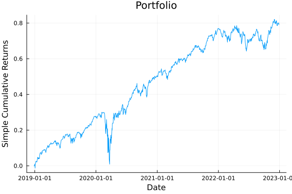
10. Summary
- A feature matrix is
assets × featuresdata carried beside the returns, not configuration held on an estimator. Static and time-varying shapes are told apart byndims. FeatureDistanceturns it into a distance, so every clustering, network and constraint consumer takes it unchanged.- Four producers supply it. Only
AssetSetsFeaturesis exogenous, which is the property the whole exercise exists for. PhylogenyFeatureshas two independent knobs on two different objects:sepchooses which pairs are related,decayhow strongly. Neither implies the other, and the default pairing hides the difference.z_srcpicks the carrier::dataslices under a fold,:priorrefits. They agree on the whole universe and diverge on a subproblem.- Cross-validation surfaces two things nothing else does — a time-varying literal cannot survive an observation fold, and a bare
PathLength()makes the scale ofZfollow the sample.
This page was generated using Literate.jl.