The source files can be found in examples/.
Profile: institutional
The third profile is an institutional mandate — a large, benchmarked book hemmed in by rules. Where the retail profile optimised for cost and the desk profile optimised for a view, this one optimises within constraints: concentration limits, sector caps, and a tracking-error budget against a benchmark. The size makes exact execution worthwhile.
The reasoning, following the strategy decision framework:
- The mandate is the boss — per-name caps, sector limits, and a benchmark tracking-error ceiling are hard requirements, exactly what the
JuMPOptimiserconstraint keywords express. - Benchmarked — this is enhanced indexing: minimise risk but stay within a tracking-error budget of the benchmark (see Turnover and Tracking).
- Large and precise — a big book justifies an exact
DiscreteAllocation.
This is the template for a constrained, benchmarked institutional book: stack the mandate's rules as JuMPOptimiser keywords, bound tracking error to the benchmark, and allocate exactly. The constraints, not the prior, are doing most of the work.
using PortfolioOptimisers, CSV, TimeSeries, DataFrames, PrettyTables, Clarabel, HiGHS, StatsPlots, GraphRecipesresfmt = (v, i, j) -> begin return if j == 1 v else isa(v, AbstractFloat) ? "$(round(v*100, digits=3)) %" : v endend;1. Data, benchmark, and groups
The benchmark is an equal-weight book; the sectors are named so the mandate's sector caps can reference them.
X = TimeArray(CSV.File(joinpath(@__DIR__, "..", "SP500.csv.gz")); timestamp = :Date)[(end - 252):end]rd = prices_to_returns(X)pr = prior(EmpiricalPrior(), rd)N = length(rd.nx)prices = vec(values(X)[end, :])benchmark = fill(1 / N, N)sets = UniverseSets(; dict = Dict("nx" => rd.nx, "tech" => ["AAPL", "AMD", "MSFT"], "energy" => ["CVX", "XOM", "RRC"], "healthcare" => ["JNJ", "LLY", "MRK", "PFE", "UNH"]))slv = Solver(; name = :clarabel, solver = Clarabel.Optimizer, settings = Dict("verbose" => false), check_sol = (; allow_local = true, allow_almost = true))Solver
name ┼ Symbol: :clarabel
solver ┼ UnionAll: Clarabel.MOIwrapper.Optimizer
settings ┼ Dict{String, Bool}: Dict{String, Bool}("verbose" => 0)
check_sol ┼ @NamedTuple{allow_local::Bool, allow_almost::Bool}: (allow_local = true, allow_almost = true)
add_bridges ┴ Bool: true
2. The constrained optimisation
Minimum risk, subject to the full mandate: a 10% per-name cap, an energy sector limit, and a tracking-error budget against the benchmark. Every rule is a keyword on the JuMPOptimiser.
institutional = optimise(MeanRisk(; obj = MinimumRisk(), opt = JuMPOptimiser(; pe = pr, slv = slv, sets = sets, wb = WeightBounds(; lb = 0.0, ub = 0.10), lcse = LinearConstraintEstimator(; val = ["energy <= 0.2"]), tr = TrackingError(; tr = WeightsTracking(; w = benchmark), err = 0.005))))sector_weight(w, g) = sum(w[i] for i in eachindex(w) if rd.nx[i] in sets.dict[g])pretty_table(DataFrame("Sector" => ["tech", "energy", "healthcare"], "Benchmark" => [sector_weight(benchmark, g) for g in ["tech", "energy", "healthcare"]], "Mandate book" => [sector_weight(institutional.w, g) for g in ["tech", "energy", "healthcare"]]); formatters = [resfmt], title = "Institutional book — capped, energy-limited, benchmark-tracking")Institutional book — capped, energy-limited, benchmark-tracking
┌────────────┬───────────┬──────────────┐
│ Sector │ Benchmark │ Mandate book │
│ String │ Float64 │ Float64 │
├────────────┼───────────┼──────────────┤
│ tech │ 15.0 % │ 2.818 % │
│ energy │ 15.0 % │ 15.002 % │
│ healthcare │ 25.0 % │ 28.487 % │
└────────────┴───────────┴──────────────┘The book respects every rule: no name above 10%, energy under its cap, and the whole portfolio stays within the tracking-error budget of the benchmark — diversified by construction rather than by a single objective.
3. Exact finite allocation
On a $10,000,000 book, DiscreteAllocation with a MIP solver (HiGHS) turns the target into whole shares with negligible residual cash.
mip_slv = Solver(; name = :highs, solver = HiGHS.Optimizer, settings = Dict("log_to_console" => false))alloc = optimise(DiscreteAllocation(; slv = mip_slv), FiniteAllocationInput(; w = institutional.w, prices = prices, cash = 10_000_000.0))invested = sum(alloc.shares .* prices)pretty_table(DataFrame("Asset" => rd.nx, "Target" => institutional.w, "Shares" => round.(Int, alloc.shares), "Realised" => alloc.w); formatters = [resfmt], title = "\$10,000,000 allocated — invested \```math(round(Int, invested)), cash left \```(round(alloc.cash, digits = 2))")$10,000,000 allocated — invested ```math(round(Int, invested)), cash left ```(round(alloc.cash, digits = 2))
┌────────┬─────────┬────────┬──────────┐
│ Asset │ Target │ Shares │ Realised │
│ String │ Float64 │ Int64 │ Float64 │
├────────┼─────────┼────────┼──────────┤
│ AAPL │ 0.0 % │ 0 │ 0.0 % │
│ AMD │ 0.0 % │ 0 │ 0.0 % │
│ BAC │ 0.0 % │ 1 │ 0.0 % │
│ BBY │ 0.0 % │ 0 │ 0.0 % │
│ CVX │ 9.999 % │ 5756 │ 10.0 % │
│ GE │ 4.039 % │ 6322 │ 4.039 % │
│ HD │ 3.983 % │ 1280 │ 3.984 % │
│ JNJ │ 10.0 % │ 5744 │ 9.999 % │
│ JPM │ 6.76 % │ 5217 │ 6.76 % │
│ KO │ 10.0 % │ 15972 │ 10.0 % │
│ LLY │ 2.603 % │ 717 │ 2.603 % │
│ MRK │ 10.0 % │ 9126 │ 10.0 % │
│ MSFT │ 2.818 % │ 1207 │ 2.818 % │
│ PEP │ 10.0 % │ 5578 │ 10.0 % │
│ PFE │ 3.219 % │ 6536 │ 3.219 % │
│ PG │ 9.855 % │ 6608 │ 9.855 % │
│ RRC │ 0.24 % │ 981 │ 0.24 % │
│ UNH │ 2.664 % │ 508 │ 2.664 % │
│ WMT │ 9.056 % │ 6460 │ 9.056 % │
│ XOM │ 4.763 % │ 4467 │ 4.763 % │
└────────┴─────────┴────────┴──────────┘4. The book
plot_stacked_bar_composition([institutional], rd; xticks = (1:1, ["Institutional"]))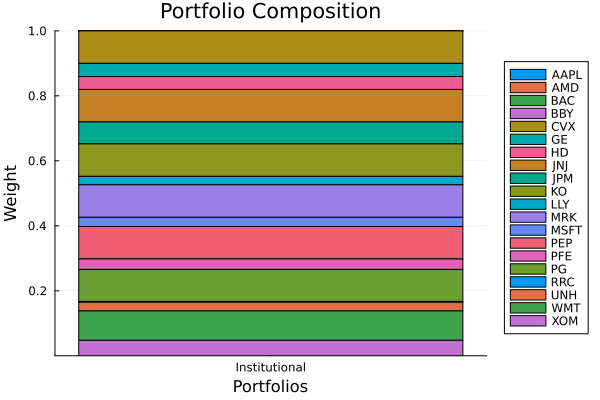
This page was generated using Literate.jl.