The source files can be found in examples/.
Clustering optimisers
The optimisers we have met so far (MeanRisk, RiskBudgeting, NearOptimalCentering) all solve a single global problem over every asset at once. Clustering optimisers take a different route: they first group the assets into a hierarchy from their dependency structure (a dendrogram), then allocate within and across those groups. Because they never invert the full covariance matrix and need no expected returns, they are robust to estimation error and require no numerical solver for variance-based risk.
PortfolioOptimisers ships three members of this family:
HierarchicalRiskParity(HRP) — recursive bisection of the dendrogram, splitting risk between each pair of sub-clusters.HierarchicalEqualRiskContribution(HERC) — equalises risk contributions both within each cluster (inner) and across clusters (outer), with independent risk measures and scalarisers for each level.SchurComplementHierarchicalRiskParity(SCHRP) — augments each sub-cluster's covariance with a Schur-complement correction, interpolating between HRP (gamma = 0) and a Markowitz-like allocation asgamma → 1.
Reach for a clustering optimiser when you want the allocation driven by the correlation structure of the assets rather than by a return forecast — to diversify across genuine groupings, to stay robust when the covariance matrix is noisy or near-singular, or simply to avoid running a solver. Use HRP for the classic robust baseline, HERC when you want explicit control of the risk split within vs across clusters, and SCHRP when you want to dial in some of mean-variance's efficiency without giving up the hierarchy's stability. If you want an explicit return/risk trade-off instead, use MeanRisk.
using PortfolioOptimisers, PrettyTables# Format for pretty tables.tsfmt = (v, i, j) -> begin if j == 1 return Date(v) else return v endend;resfmt = (v, i, j) -> begin if j == 1 return v else return isa(v, Number) ? "$(round(v*100, digits=3)) %" : v endend;1. ReturnsResult data
We use the same S&P 500 slice as the other optimiser examples.
using CSV, TimeSeries, DataFramesX = TimeArray(CSV.File(joinpath(@__DIR__, "..", "SP500.csv.gz")); timestamp = :Date)[(end - 252):end]pretty_table(X[(end - 5):end]; formatters = [tsfmt])# Compute the returnsrd = prices_to_returns(X)ReturnsResult
nx ┼ 20-element Vector{String}
X ┼ 252×20 Matrix{Float64}
nf ┼ nothing
F ┼ nothing
nb ┼ nothing
B ┼ nothing
ts ┼ 252-element Vector{Date}
iv ┼ nothing
ivpa ┼ nothing
nz ┼ nothing
Z ┴ nothing
2. Prior and clustering
Clustering optimisers need two precomputable ingredients: a prior (for the covariance) and a clustering of the assets. We compute both once and reuse them across every optimiser so the comparison is apples-to-apples — only the allocation algorithm changes.
We cluster with the Direct Bubble Hierarchy Tree (DBHT) algorithm, which builds the hierarchy from the correlation-derived distance matrix.
pr = prior(EmpiricalPrior(), rd)clr = clusterise(ClustersEstimator(; alg = DBHT()), pr.X)Clusters
res ┼ Clustering.Hclust{Float64}([-1 -13; -7 -4; … ; 12 17; 10 18], [0.1, 0.1111111111111111, 0.125, 0.14285714285714285, 0.16666666666666666, 0.2, 0.25, 0.3333333333333333, 0.5, 1.0, 0.125, 0.14285714285714285, 0.16666666666666666, 0.2, 0.25, 0.3333333333333333, 0.5, 1.0, 2.0], [5, 20, 17, 3, 9, 6, 2, 1, 13, 7, 4, 19, 14, 10, 16, 18, 11, 8, 12, 15], :DBHT)
S ┼ 20×20 Matrix{Float64}
D ┼ 20×20 Matrix{Float64}
P ┼ nothing
k ┴ Int64: 4
We can inspect the structure the optimisers will act on: the dendrogram and the reordered correlation heatmap with the detected cluster boundaries.
Hierarchical clustering dendrogram.
using StatsPlots, GraphRecipesReordered correlation heatmap with cluster boundary boxes.
plot_dendrogram(clr, rd.nx)plot_clusters(clr, rd.nx)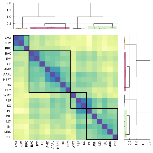
3. Hierarchical risk parity (HRP)
HRP recursively bisects the dendrogram and splits the budget between each pair of sub-clusters in inverse proportion to their risk. We pass the shared prior and clustering through a HierarchicalOptimiser. Variance needs no solver, so none is supplied.
opt = HierarchicalOptimiser(; pe = pr, cle = clr)res_hrp = optimise(HierarchicalRiskParity(; opt = opt, r = Variance()))HierarchicalRiskParityResult
hr ┼ HierarchicalResult
│ pr ┼ LowOrderPrior
│ │ X ┼ 252×20 Matrix{Float64}
│ │ o_X ┼ nothing
│ │ mu ┼ 20-element Vector{Float64}
│ │ sigma ┼ 20×20 Matrix{Float64}
│ │ chol ┼ nothing
│ │ w ┼ nothing
│ │ ens ┼ nothing
│ │ kld ┼ nothing
│ │ ow ┼ nothing
│ │ rr ┼ nothing
│ │ fpr ┼ nothing
│ │ Z ┴ nothing
│ clr ┼ Clusters
│ │ res ┼ Clustering.Hclust{Float64}([-1 -13; -7 -4; … ; 12 17; 10 18], [0.1, 0.1111111111111111, 0.125, 0.14285714285714285, 0.16666666666666666, 0.2, 0.25, 0.3333333333333333, 0.5, 1.0, 0.125, 0.14285714285714285, 0.16666666666666666, 0.2, 0.25, 0.3333333333333333, 0.5, 1.0, 2.0], [5, 20, 17, 3, 9, 6, 2, 1, 13, 7, 4, 19, 14, 10, 16, 18, 11, 8, 12, 15], :DBHT)
│ │ S ┼ 20×20 Matrix{Float64}
│ │ D ┼ 20×20 Matrix{Float64}
│ │ P ┼ nothing
│ │ k ┴ Int64: 4
│ wb ┼ WeightBounds
│ │ lb ┼ 20-element StepRangeLen{Float64, Base.TwicePrecision{Float64}, Base.TwicePrecision{Float64}, Int64}
│ │ ub ┴ 20-element StepRangeLen{Float64, Base.TwicePrecision{Float64}, Base.TwicePrecision{Float64}, Int64}
│ fees ┼ nothing
│ retcode ┼ OptimisationSuccess
│ │ res ┴ nothing
│ w ┴ 20-element Vector{Float64}
r ┼ Variance
│ settings ┼ RiskMeasureSettings
│ │ scale ┼ Float64: 1.0
│ │ ub ┼ nothing
│ │ rke ┴ Bool: true
│ sigma ┼ 20×20 Matrix{Float64}
│ chol ┼ nothing
│ rc ┼ nothing
│ alg ┴ SquaredSOCRiskExpr()
sca ┼ SumScalariser()
fb ┴ nothing
4. Hierarchical equal risk contribution (HERC)
HERC equalises risk contributions within each cluster (the inner problem) and across clusters (the outer problem). It accepts separate inner/outer risk measures (ri, ro) and scalarisers (scai, scao); here we use Variance for both levels.
res_herc = optimise(HierarchicalEqualRiskContribution(; opt = opt, ri = Variance(), ro = Variance()))HierarchicalEqualRiskContributionResult
hr ┼ HierarchicalResult
│ pr ┼ LowOrderPrior
│ │ X ┼ 252×20 Matrix{Float64}
│ │ o_X ┼ nothing
│ │ mu ┼ 20-element Vector{Float64}
│ │ sigma ┼ 20×20 Matrix{Float64}
│ │ chol ┼ nothing
│ │ w ┼ nothing
│ │ ens ┼ nothing
│ │ kld ┼ nothing
│ │ ow ┼ nothing
│ │ rr ┼ nothing
│ │ fpr ┼ nothing
│ │ Z ┴ nothing
│ clr ┼ Clusters
│ │ res ┼ Clustering.Hclust{Float64}([-1 -13; -7 -4; … ; 12 17; 10 18], [0.1, 0.1111111111111111, 0.125, 0.14285714285714285, 0.16666666666666666, 0.2, 0.25, 0.3333333333333333, 0.5, 1.0, 0.125, 0.14285714285714285, 0.16666666666666666, 0.2, 0.25, 0.3333333333333333, 0.5, 1.0, 2.0], [5, 20, 17, 3, 9, 6, 2, 1, 13, 7, 4, 19, 14, 10, 16, 18, 11, 8, 12, 15], :DBHT)
│ │ S ┼ 20×20 Matrix{Float64}
│ │ D ┼ 20×20 Matrix{Float64}
│ │ P ┼ nothing
│ │ k ┴ Int64: 4
│ wb ┼ WeightBounds
│ │ lb ┼ 20-element StepRangeLen{Float64, Base.TwicePrecision{Float64}, Base.TwicePrecision{Float64}, Int64}
│ │ ub ┴ 20-element StepRangeLen{Float64, Base.TwicePrecision{Float64}, Base.TwicePrecision{Float64}, Int64}
│ fees ┼ nothing
│ retcode ┼ OptimisationSuccess
│ │ res ┴ nothing
│ w ┴ 20-element Vector{Float64}
ri ┼ Variance
│ settings ┼ RiskMeasureSettings
│ │ scale ┼ Float64: 1.0
│ │ ub ┼ nothing
│ │ rke ┴ Bool: true
│ sigma ┼ 20×20 Matrix{Float64}
│ chol ┼ nothing
│ rc ┼ nothing
│ alg ┴ SquaredSOCRiskExpr()
ro ┼ Variance
│ settings ┼ RiskMeasureSettings
│ │ scale ┼ Float64: 1.0
│ │ ub ┼ nothing
│ │ rke ┴ Bool: true
│ sigma ┼ 20×20 Matrix{Float64}
│ chol ┼ nothing
│ rc ┼ nothing
│ alg ┴ SquaredSOCRiskExpr()
scai ┼ SumScalariser()
scao ┼ SumScalariser()
fb ┴ nothing
5. Schur-complement HRP (SCHRP)
SCHRP corrects each sub-cluster's covariance with a Schur complement of the off-diagonal (inter-cluster) block, controlled by gamma. At gamma = 0 it reduces to HRP; as gamma grows it absorbs more of the cross-cluster information, moving toward a Markowitz-like allocation while keeping the hierarchical structure. We sweep three values to make the interpolation visible.
res_schur0 = optimise(SchurComplementHierarchicalRiskParity(; opt = opt, params = SchurComplementParams(; r = Variance(), gamma = 0.0)))res_schur5 = optimise(SchurComplementHierarchicalRiskParity(; opt = opt, params = SchurComplementParams(; r = Variance(), gamma = 0.5)))res_schur9 = optimise(SchurComplementHierarchicalRiskParity(; opt = opt, params = SchurComplementParams(; r = Variance(), gamma = 0.9)))SchurComplementHierarchicalRiskParityResult
pr ┼ LowOrderPrior
│ X ┼ 252×20 Matrix{Float64}
│ o_X ┼ nothing
│ mu ┼ 20-element Vector{Float64}
│ sigma ┼ 20×20 Matrix{Float64}
│ chol ┼ nothing
│ w ┼ nothing
│ ens ┼ nothing
│ kld ┼ nothing
│ ow ┼ nothing
│ rr ┼ nothing
│ fpr ┼ nothing
│ Z ┴ nothing
wb ┼ WeightBounds
│ lb ┼ 20-element StepRangeLen{Float64, Base.TwicePrecision{Float64}, Base.TwicePrecision{Float64}, Int64}
│ ub ┴ 20-element StepRangeLen{Float64, Base.TwicePrecision{Float64}, Base.TwicePrecision{Float64}, Int64}
clr ┼ Clusters
│ res ┼ Clustering.Hclust{Float64}([-1 -13; -7 -4; … ; 12 17; 10 18], [0.1, 0.1111111111111111, 0.125, 0.14285714285714285, 0.16666666666666666, 0.2, 0.25, 0.3333333333333333, 0.5, 1.0, 0.125, 0.14285714285714285, 0.16666666666666666, 0.2, 0.25, 0.3333333333333333, 0.5, 1.0, 2.0], [5, 20, 17, 3, 9, 6, 2, 1, 13, 7, 4, 19, 14, 10, 16, 18, 11, 8, 12, 15], :DBHT)
│ S ┼ 20×20 Matrix{Float64}
│ D ┼ 20×20 Matrix{Float64}
│ P ┼ nothing
│ k ┴ Int64: 4
r ┼ Variance
│ settings ┼ RiskMeasureSettings
│ │ scale ┼ Float64: 1.0
│ │ ub ┼ nothing
│ │ rke ┴ Bool: true
│ sigma ┼ 20×20 Matrix{Float64}
│ chol ┼ nothing
│ rc ┼ nothing
│ alg ┴ SquaredSOCRiskExpr()
gamma ┼ Float64: 0.10087890625000001
retcode ┼ OptimisationSuccess
│ res ┴ nothing
w ┼ 20-element Vector{Float64}
fb ┴ nothing
6. Comparing the allocations
With everything sharing one prior and one clustering, the weight differences come purely from the allocation rule. Note how SCHRP at gamma = 0 matches HRP, and drifts away from it as gamma increases.
pretty_table(DataFrame(; :assets => rd.nx, :HRP => res_hrp.w, :HERC => res_herc.w, Symbol("SCHRP γ=0") => res_schur0.w, Symbol("SCHRP γ=0.5") => res_schur5.w, Symbol("SCHRP γ=0.9") => res_schur9.w); formatters = [resfmt])┌────────┬──────────┬──────────┬───────────┬─────────────┬─────────────┐
│ assets │ HRP │ HERC │ SCHRP γ=0 │ SCHRP γ=0.5 │ SCHRP γ=0.9 │
│ String │ Float64 │ Float64 │ Float64 │ Float64 │ Float64 │
├────────┼──────────┼──────────┼───────────┼─────────────┼─────────────┤
│ AAPL │ 3.26 % │ 1.847 % │ 3.26 % │ 3.257 % │ 3.257 % │
│ AMD │ 1.263 % │ 0.627 % │ 1.263 % │ 1.285 % │ 1.285 % │
│ BAC │ 3.356 % │ 2.221 % │ 3.356 % │ 3.206 % │ 3.207 % │
│ BBY │ 2.871 % │ 1.138 % │ 2.871 % │ 2.912 % │ 2.912 % │
│ CVX │ 3.937 % │ 4.525 % │ 3.937 % │ 3.915 % │ 3.915 % │
│ GE │ 3.879 % │ 1.924 % │ 3.879 % │ 3.769 % │ 3.769 % │
│ HD │ 2.605 % │ 2.386 % │ 2.605 % │ 2.606 % │ 2.606 % │
│ JNJ │ 13.136 % │ 10.746 % │ 13.136 % │ 13.011 % │ 13.011 % │
│ JPM │ 3.965 % │ 2.623 % │ 3.965 % │ 3.812 % │ 3.812 % │
│ KO │ 6.299 % │ 13.86 % │ 6.299 % │ 6.35 % │ 6.35 % │
│ LLY │ 5.995 % │ 4.388 % │ 5.995 % │ 6.209 % │ 6.209 % │
│ MRK │ 6.583 % │ 8.205 % │ 6.583 % │ 6.451 % │ 6.452 % │
│ MSFT │ 2.06 % │ 1.886 % │ 2.06 % │ 2.087 % │ 2.087 % │
│ PEP │ 11.24 % │ 14.175 % │ 11.24 % │ 11.416 % │ 11.416 % │
│ PFE │ 3.589 % │ 4.473 % │ 3.589 % │ 3.447 % │ 3.447 % │
│ PG │ 5.051 % │ 6.756 % │ 5.051 % │ 5.118 % │ 5.118 % │
│ RRC │ 1.691 % │ 1.238 % │ 1.691 % │ 1.589 % │ 1.589 % │
│ UNH │ 7.499 % │ 5.489 % │ 7.499 % │ 7.788 % │ 7.788 % │
│ WMT │ 8.257 % │ 7.513 % │ 8.257 % │ 8.332 % │ 8.332 % │
│ XOM │ 3.464 % │ 3.98 % │ 3.464 % │ 3.44 % │ 3.44 % │
└────────┴──────────┴──────────┴───────────┴─────────────┴─────────────┘The composition plot shows the same story visually across the five allocations.
plot_stacked_bar_composition([res_hrp, res_herc, res_schur0, res_schur5, res_schur9], rd)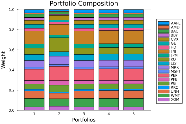
Finally, the per-asset variance risk contributions for the HRP portfolio confirm that risk — not capital — is what the hierarchy spreads out. The risk measure needs its covariance populated from the prior first, which is what factory does.
rv = factory(Variance(), pr)plot_risk_contribution(rv, res_hrp, rd)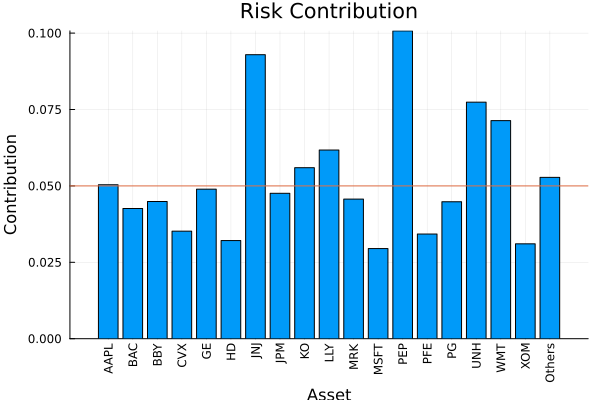
This page was generated using Literate.jl.