The source files can be found in examples/.
Efficient frontier
A single MeanRisk optimisation returns one portfolio. The efficient frontier is the whole curve of portfolios that earn the most return for each level of risk. They are also the portfolios that take the least risk for each level of return. You compute the whole trade-off first, and then choose a point on it.
This page adds three things to the MeanRisk objectives page. It computes the frontier from both directions, once by minimising risk above a return floor and once by maximising return below a risk ceiling, and plots the two on one chart. It introduces Frontier, which finds the bounds of the frontier for you. It then compares the MeanRisk frontier with the centred frontier of NearOptimalCentering, which gives up a little of the objective for a portfolio that holds more assets at each point.
Reach for an efficient frontier when you do not want to fix one point of risk and return in advance. You see the whole curve and choose a portfolio on it, or pass its points to a rule that selects one. Read the MeanRisk objectives page first, since each point of a frontier is one of those optimisations. For more than two criteria, see the Pareto surface example.
using PortfolioOptimisers, PrettyTablestsfmt = (v, i, j) -> begin if j == 1 return Date(v) else return v endend;resfmt = (v, i, j) -> begin if j == 1 return v else return isa(v, Number) ? "$(round(v*100, digits=3)) %" : v endend;1. Data
We use the same data as the previous example.
using CSV, TimeSeries, DataFramesX = TimeArray(CSV.File(joinpath(@__DIR__, "..", "SP500.csv.gz")); timestamp = :Date)[(end - 252):end]pretty_table(X[(end - 5):end]; formatters = [tsfmt])rd = prices_to_returns(X)ReturnsResult
nx ┼ 20-element Vector{String}
X ┼ 252×20 Matrix{Float64}
nf ┼ nothing
F ┼ nothing
nb ┼ nothing
B ┼ nothing
ne ┼ nothing
E ┼ nothing
ts ┼ 252-element Vector{Date}
iv ┼ nothing
ivpa ┼ nothing
pnl ┼ AssetPanel
│ pf ┼ Vector{AbstractPanelField}: AbstractPanelField[]
│ amsk ┼ 252×20 AllTrueMask
│ emsk ┴ 252×20 AllTrueMask
2. Two directions, four combinations
You compute a frontier in one of two directions.
- Minimise risk with a lower bound on the return, and raise the bound from point to point.
- Maximise return with an upper bound on the risk, and raise the bound from point to point.
Each bound can be a range of numbers that you choose, or a Frontier, which finds the lowest and the highest feasible value and spaces the points between them. Two directions and two kinds of bound give four combinations, and this page uses Frontier in both directions. The two directions give the same curve, so choose the one whose quantity is easier to set in your problem.
We use the conditional value at risk (CVaR), ConditionalValueatRisk, as the risk measure on the whole page, and compute the prior once and share it across every optimisation. One solver setting can fail to converge at some points of a frontier, so we pass a vector of two solvers. When the first fails, the optimiser tries the second.
using Clarabelslv = [Solver(; name = :clarabel1, solver = Clarabel.Optimizer, settings = Dict("verbose" => false), check_sol = (; allow_local = true, allow_almost = true)), Solver(; name = :clarabel2, solver = Clarabel.Optimizer, settings = Dict("verbose" => false, "max_step_fraction" => 0.75), check_sol = (; allow_local = true, allow_almost = true))]r = ConditionalValueatRisk()pr = prior(EmpiricalPrior(), rd)rf = 4.2 / 100 / 2520.0001666666666666667Direction A: minimise risk above a return floor
We set no objective, so the optimisation takes the default, MinimumRisk, and minimises the CVaR. A Frontier of 30 points sets the lower bound on the return. The bound is on the return, so it goes in the settings of ArithmeticReturn, as lb.
optA = JuMPOptimiser(; pe = pr, slv = slv, ret = ArithmeticReturn(; settings = JuMPReturnsSettings(; lb = Frontier(; N = 30))))resA = optimise(MeanRisk(; opt = optA, r = r))MeanRiskResult
jr ┼ JuMPOptimisationResult
│ pa ┼ ProcessedJuMPOptimiserAttributes
│ │ pr ┼ LowOrderPrior
│ │ │ X ┼ 252×20 Matrix{Float64}
│ │ │ o_X ┼ nothing
│ │ │ mu ┼ 20-element Vector{Float64}
│ │ │ sigma ┼ 20×20 Matrix{Float64}
│ │ │ chol ┼ nothing
│ │ │ w ┼ nothing
│ │ │ ens ┼ nothing
│ │ │ kld ┼ nothing
│ │ │ ow ┼ nothing
│ │ │ rr ┼ nothing
│ │ │ fpr ┼ nothing
│ │ │ x_src ┼ nothing
│ │ │ ss_gaps ┼ nothing
│ │ │ pc ┴ nothing
│ │ wb ┼ WeightBounds
│ │ │ lb ┼ 20-element StepRangeLen{Float64, Base.TwicePrecision{Float64}, Base.TwicePrecision{Float64}, Int64}
│ │ │ ub ┴ 20-element StepRangeLen{Float64, Base.TwicePrecision{Float64}, Base.TwicePrecision{Float64}, Int64}
│ │ lt ┼ nothing
│ │ st ┼ nothing
│ │ lcsr ┼ nothing
│ │ ctr ┼ nothing
│ │ gcardr ┼ nothing
│ │ sgcardr ┼ nothing
│ │ smtx ┼ nothing
│ │ sgmtx ┼ nothing
│ │ slt ┼ nothing
│ │ sst ┼ nothing
│ │ sglt ┼ nothing
│ │ sgst ┼ nothing
│ │ tn ┼ nothing
│ │ fees ┼ nothing
│ │ plr ┼ nothing
│ │ ret ┼ ArithmeticReturn
│ │ │ settings ┼ JuMPReturnsSettings
│ │ │ │ scale ┼ Float64: 1.0
│ │ │ │ lb ┼ Frontier
│ │ │ │ │ N ┼ Int64: 30
│ │ │ │ │ factor ┼ Int64: 1
│ │ │ │ │ bound ┴ LinearBound()
│ │ │ │ rte ┼ Bool: true
│ │ │ │ fee ┼ Bool: true
│ │ │ │ mic ┴ Bool: true
│ │ │ ucs ┼ nothing
│ │ │ mu ┼ 20-element Vector{Float64}
│ │ │ mtx_sqrt ┴ EigenFallbackSquareRoot()
│ │ sca ┼ SumScalariser()
│ │ imsk ┴ nothing
│ retcode ┼ 30-element Vector{OptimisationSuccess}
│ │ OptimisationSuccess ⋯
│ │ OptimisationSuccess ⋯
│ │ OptimisationSuccess ⋯
│ │ OptimisationSuccess ⋯
│ │ OptimisationSuccess ⋯
│ │ OptimisationSuccess ⋯
│ │ OptimisationSuccess ⋯
│ │ OptimisationSuccess ⋯
│ │ OptimisationSuccess ⋯
│ │ OptimisationSuccess ⋯
│ │ OptimisationSuccess ⋯
│ │ OptimisationSuccess ⋯
│ │ OptimisationSuccess ⋯
│ │ OptimisationSuccess ⋯
│ │ OptimisationSuccess ⋯
│ │ OptimisationSuccess ⋯
│ │ OptimisationSuccess ⋯
│ │ OptimisationSuccess ⋯
│ │ OptimisationSuccess ⋯
│ │ OptimisationSuccess ⋯
│ │ OptimisationSuccess ⋯
│ │ OptimisationSuccess ⋯
│ │ OptimisationSuccess ⋯
│ │ OptimisationSuccess ⋯
│ │ OptimisationSuccess ⋯
│ │ OptimisationSuccess ⋯
│ │ OptimisationSuccess ⋯
│ │ OptimisationSuccess ⋯
│ │ OptimisationSuccess ⋯
│ │ OptimisationSuccess ⋯
│ sol ┼ 30-element Vector{JuMPOptimisationSolution}
│ │ JuMPOptimisationSolution ⋯
│ │ JuMPOptimisationSolution ⋯
│ │ JuMPOptimisationSolution ⋯
│ │ JuMPOptimisationSolution ⋯
│ │ JuMPOptimisationSolution ⋯
│ │ JuMPOptimisationSolution ⋯
│ │ JuMPOptimisationSolution ⋯
│ │ JuMPOptimisationSolution ⋯
│ │ JuMPOptimisationSolution ⋯
│ │ JuMPOptimisationSolution ⋯
│ │ JuMPOptimisationSolution ⋯
│ │ JuMPOptimisationSolution ⋯
│ │ JuMPOptimisationSolution ⋯
│ │ JuMPOptimisationSolution ⋯
│ │ JuMPOptimisationSolution ⋯
│ │ JuMPOptimisationSolution ⋯
│ │ JuMPOptimisationSolution ⋯
│ │ JuMPOptimisationSolution ⋯
│ │ JuMPOptimisationSolution ⋯
│ │ JuMPOptimisationSolution ⋯
│ │ JuMPOptimisationSolution ⋯
│ │ JuMPOptimisationSolution ⋯
│ │ JuMPOptimisationSolution ⋯
│ │ JuMPOptimisationSolution ⋯
│ │ JuMPOptimisationSolution ⋯
│ │ JuMPOptimisationSolution ⋯
│ │ JuMPOptimisationSolution ⋯
│ │ JuMPOptimisationSolution ⋯
│ │ JuMPOptimisationSolution ⋯
│ │ JuMPOptimisationSolution ⋯
│ model ┼ A JuMP Model
│ │ ├ solver: Clarabel
│ │ ├ objective_sense: MIN_SENSE
│ │ │ └ objective_function_type: AffExpr
│ │ ├ num_variables: 274
│ │ ├ num_constraints: 258
│ │ │ ├ AffExpr in MOI.EqualTo{Float64}: 1
│ │ │ ├ AffExpr in MOI.GreaterThan{Float64}: 1
│ │ │ ├ Vector{AffExpr} in MOI.Nonnegatives: 2
│ │ │ ├ Vector{AffExpr} in MOI.Nonpositives: 1
│ │ │ ├ VariableRef in MOI.GreaterThan{Float64}: 252
│ │ │ └ VariableRef in MOI.Parameter{Float64}: 1
│ │ └ Names registered in the model
│ │ └ :T, :X, :bgt, :ccvar_1, :cvar_risk_1, :k, :lw, :net_X, :obj_expr, :ret, :ret_1, :ret_frontier, :ret_lb_1, :ret_lb_var_1, :ret_vec, :risk, :risk_minimised, :risk_vec, :sc, :so, :var_1, :w, :w_gross_ub, :w_lb, :w_ub, :z_cvar_1
r ┼ ConditionalValueatRisk
│ settings ┼ RiskMeasureSettings
│ │ scale ┼ Float64: 1.0
│ │ ub ┼ nothing
│ │ rke ┴ Bool: true
│ alpha ┼ Float64: 0.05
│ w ┴ nothing
fb ┴ nothing
retcode and sol now have one entry per point of the frontier. We check that every point solved.
all(x -> isa(x, OptimisationSuccess), resA.retcode)trueThe table has one column of weights per point. From point 1 to point 30 the portfolio moves from many assets at the low-risk end to few assets at the high-return end.
pretty_table(DataFrame([rd.nx hcat(resA.w...)], Symbol.([:assets; 1:30])); formatters = [resfmt])┌────────┬──────────┬──────────┬──────────┬──────────┬──────────┬──────────┬──────────┬──────────┬──────────┬──────────┬──────────┬──────────┬──────────┬──────────┬──────────┬──────────┬──────────┬──────────┬──────────┬──────────┬──────────┬──────────┬──────────┬──────────┬──────────┬──────────┬──────────┬─────────┬─────────┬─────────┐
│ assets │ 1 │ 2 │ 3 │ 4 │ 5 │ 6 │ 7 │ 8 │ 9 │ 10 │ 11 │ 12 │ 13 │ 14 │ 15 │ 16 │ 17 │ 18 │ 19 │ 20 │ 21 │ 22 │ 23 │ 24 │ 25 │ 26 │ 27 │ 28 │ 29 │ 30 │
│ Any │ Any │ Any │ Any │ Any │ Any │ Any │ Any │ Any │ Any │ Any │ Any │ Any │ Any │ Any │ Any │ Any │ Any │ Any │ Any │ Any │ Any │ Any │ Any │ Any │ Any │ Any │ Any │ Any │ Any │ Any │
├────────┼──────────┼──────────┼──────────┼──────────┼──────────┼──────────┼──────────┼──────────┼──────────┼──────────┼──────────┼──────────┼──────────┼──────────┼──────────┼──────────┼──────────┼──────────┼──────────┼──────────┼──────────┼──────────┼──────────┼──────────┼──────────┼──────────┼──────────┼─────────┼─────────┼─────────┤
│ AAPL │ 0.0 % │ 0.0 % │ 0.0 % │ 0.0 % │ 0.0 % │ 0.0 % │ 0.0 % │ 0.0 % │ 0.0 % │ 0.0 % │ 0.0 % │ 0.0 % │ 0.0 % │ 0.0 % │ 0.0 % │ 0.0 % │ 0.0 % │ 0.0 % │ 0.0 % │ 0.0 % │ 0.0 % │ 0.0 % │ 0.0 % │ 0.0 % │ 0.0 % │ 0.0 % │ 0.0 % │ 0.0 % │ 0.0 % │ 0.0 % │
│ AMD │ 0.0 % │ 0.0 % │ 0.0 % │ 0.0 % │ 0.0 % │ 0.0 % │ 0.0 % │ 0.0 % │ 0.0 % │ 0.0 % │ 0.0 % │ 0.0 % │ 0.0 % │ 0.0 % │ 0.0 % │ 0.0 % │ 0.0 % │ 0.0 % │ 0.0 % │ 0.0 % │ 0.0 % │ 0.0 % │ -0.0 % │ -0.0 % │ -0.0 % │ -0.0 % │ -0.0 % │ -0.0 % │ -0.0 % │ -0.0 % │
│ BAC │ 0.0 % │ 0.0 % │ 0.0 % │ 0.0 % │ 0.0 % │ 0.0 % │ 0.0 % │ 0.0 % │ 0.0 % │ 0.0 % │ 0.0 % │ 0.0 % │ 0.0 % │ 0.0 % │ 0.0 % │ 0.0 % │ 0.0 % │ 0.0 % │ 0.0 % │ 0.0 % │ 0.0 % │ 0.0 % │ 0.0 % │ 0.0 % │ 0.0 % │ 0.0 % │ 0.0 % │ 0.0 % │ 0.0 % │ 0.0 % │
│ BBY │ 0.0 % │ 0.0 % │ 0.0 % │ 0.0 % │ 0.0 % │ 0.0 % │ 0.0 % │ 0.0 % │ 0.0 % │ 0.0 % │ 0.0 % │ 0.0 % │ 0.0 % │ 0.0 % │ 0.0 % │ 0.0 % │ 0.0 % │ 0.0 % │ 0.0 % │ 0.0 % │ 0.0 % │ 0.0 % │ 0.0 % │ 0.0 % │ 0.0 % │ 0.0 % │ 0.0 % │ 0.0 % │ 0.0 % │ 0.0 % │
│ CVX │ 13.167 % │ 12.757 % │ 9.552 % │ 3.037 % │ 1.821 % │ 0.159 % │ 0.0 % │ 0.0 % │ 0.0 % │ 0.0 % │ 0.0 % │ 0.0 % │ 0.0 % │ 0.0 % │ 0.0 % │ 0.0 % │ 0.0 % │ 0.0 % │ 0.0 % │ 0.0 % │ 0.0 % │ 0.0 % │ 0.0 % │ 0.0 % │ 0.0 % │ 0.0 % │ 0.0 % │ 0.0 % │ 0.0 % │ 0.0 % │
│ GE │ 0.0 % │ 0.0 % │ 0.0 % │ 0.0 % │ 0.0 % │ 0.0 % │ 0.0 % │ 0.0 % │ 0.0 % │ 0.0 % │ 0.0 % │ 0.0 % │ 0.0 % │ 0.0 % │ 0.0 % │ 0.0 % │ 0.0 % │ 0.0 % │ 0.0 % │ 0.0 % │ 0.0 % │ 0.0 % │ 0.0 % │ 0.0 % │ 0.0 % │ 0.0 % │ 0.0 % │ 0.0 % │ 0.0 % │ 0.0 % │
│ HD │ 0.0 % │ 0.0 % │ 0.0 % │ 0.0 % │ 0.0 % │ 0.0 % │ 0.0 % │ 0.0 % │ 0.0 % │ 0.0 % │ 0.0 % │ 0.0 % │ 0.0 % │ 0.0 % │ 0.0 % │ 0.0 % │ 0.0 % │ 0.0 % │ 0.0 % │ 0.0 % │ 0.0 % │ 0.0 % │ 0.0 % │ 0.0 % │ 0.0 % │ 0.0 % │ 0.0 % │ 0.0 % │ 0.0 % │ 0.0 % │
│ JNJ │ 45.342 % │ 40.238 % │ 37.261 % │ 32.596 % │ 29.384 % │ 26.772 % │ 25.171 % │ 20.067 % │ 16.324 % │ 14.245 % │ 12.166 % │ 10.087 % │ 8.008 % │ 6.101 % │ 1.996 % │ 0.0 % │ 0.0 % │ 0.0 % │ 0.0 % │ 0.0 % │ 0.0 % │ 0.0 % │ 0.0 % │ 0.0 % │ 0.0 % │ 0.0 % │ 0.0 % │ 0.0 % │ 0.0 % │ 0.0 % │
│ JPM │ 0.0 % │ 0.0 % │ 0.0 % │ 0.0 % │ 0.0 % │ 0.0 % │ 0.0 % │ 0.0 % │ 0.0 % │ 0.0 % │ 0.0 % │ 0.0 % │ 0.0 % │ 0.0 % │ 0.0 % │ 0.0 % │ 0.0 % │ 0.0 % │ 0.0 % │ 0.0 % │ 0.0 % │ 0.0 % │ 0.0 % │ 0.0 % │ 0.0 % │ 0.0 % │ 0.0 % │ 0.0 % │ 0.0 % │ 0.0 % │
│ KO │ 13.285 % │ 14.244 % │ 14.767 % │ 18.327 % │ 17.772 % │ 17.332 % │ 15.194 % │ 16.637 % │ 16.595 % │ 14.902 % │ 13.209 % │ 11.516 % │ 9.823 % │ 8.064 % │ 8.415 % │ 6.517 % │ 2.705 % │ 0.0 % │ 0.0 % │ 0.0 % │ 0.0 % │ 0.0 % │ 0.0 % │ 0.0 % │ 0.0 % │ 0.0 % │ 0.0 % │ 0.0 % │ 0.0 % │ 0.0 % │
│ LLY │ 0.0 % │ 0.0 % │ 0.0 % │ 0.0 % │ 0.0 % │ 0.0 % │ 0.0 % │ 0.0 % │ 0.0 % │ 0.0 % │ 0.0 % │ 0.0 % │ 0.0 % │ 0.0 % │ 0.0 % │ 0.0 % │ 0.0 % │ 0.0 % │ 0.0 % │ 0.0 % │ 0.0 % │ 0.0 % │ 0.0 % │ 0.0 % │ 0.0 % │ 0.0 % │ 0.0 % │ 0.0 % │ 0.0 % │ 0.0 % │
│ MRK │ 20.556 % │ 25.205 % │ 27.696 % │ 29.897 % │ 33.915 % │ 36.555 % │ 39.437 % │ 42.723 % │ 46.016 % │ 48.955 % │ 51.893 % │ 54.832 % │ 57.77 % │ 60.441 % │ 63.737 % │ 66.926 % │ 69.546 % │ 69.717 % │ 63.907 % │ 58.098 % │ 52.288 % │ 46.478 % │ 40.668 % │ 34.859 % │ 29.049 % │ 23.239 % │ 17.429 % │ 11.62 % │ 5.81 % │ 0.0 % │
│ MSFT │ 0.0 % │ 0.0 % │ 0.0 % │ 0.0 % │ 0.0 % │ 0.0 % │ 0.0 % │ 0.0 % │ 0.0 % │ 0.0 % │ 0.0 % │ 0.0 % │ 0.0 % │ 0.0 % │ 0.0 % │ 0.0 % │ 0.0 % │ 0.0 % │ 0.0 % │ 0.0 % │ 0.0 % │ 0.0 % │ 0.0 % │ 0.0 % │ 0.0 % │ 0.0 % │ 0.0 % │ 0.0 % │ 0.0 % │ 0.0 % │
│ PEP │ 0.0 % │ 0.0 % │ 0.0 % │ 0.0 % │ 0.0 % │ 0.0 % │ 0.0 % │ 0.0 % │ 0.0 % │ 0.0 % │ 0.0 % │ 0.0 % │ 0.0 % │ 0.0 % │ 0.0 % │ 0.0 % │ 0.0 % │ 0.0 % │ 0.0 % │ 0.0 % │ 0.0 % │ 0.0 % │ 0.0 % │ 0.0 % │ 0.0 % │ 0.0 % │ 0.0 % │ 0.0 % │ 0.0 % │ 0.0 % │
│ PFE │ 0.0 % │ 0.0 % │ 0.0 % │ 0.0 % │ 0.0 % │ 0.0 % │ 0.0 % │ 0.0 % │ 0.0 % │ 0.0 % │ 0.0 % │ 0.0 % │ 0.0 % │ 0.0 % │ 0.0 % │ 0.0 % │ 0.0 % │ 0.0 % │ 0.0 % │ 0.0 % │ 0.0 % │ 0.0 % │ 0.0 % │ 0.0 % │ 0.0 % │ 0.0 % │ 0.0 % │ 0.0 % │ 0.0 % │ 0.0 % │
│ PG │ 0.0 % │ 0.0 % │ 0.0 % │ 0.0 % │ 0.0 % │ 0.0 % │ 0.0 % │ 0.0 % │ 0.0 % │ 0.0 % │ 0.0 % │ 0.0 % │ 0.0 % │ 0.0 % │ 0.0 % │ 0.0 % │ 0.0 % │ 0.0 % │ 0.0 % │ 0.0 % │ 0.0 % │ 0.0 % │ 0.0 % │ 0.0 % │ 0.0 % │ 0.0 % │ 0.0 % │ 0.0 % │ 0.0 % │ 0.0 % │
│ RRC │ 0.0 % │ 0.0 % │ 0.0 % │ 0.0 % │ 0.0 % │ 0.0 % │ 0.0 % │ 0.0 % │ 0.0 % │ 0.0 % │ 0.0 % │ 0.0 % │ 0.0 % │ 0.0 % │ 0.0 % │ 0.0 % │ 0.0 % │ 0.0 % │ 0.0 % │ 0.0 % │ 0.0 % │ 0.0 % │ 0.0 % │ 0.0 % │ 0.0 % │ 0.0 % │ 0.0 % │ 0.0 % │ 0.0 % │ 0.0 % │
│ UNH │ 0.0 % │ 0.0 % │ 0.0 % │ 0.0 % │ 0.0 % │ 0.0 % │ 0.0 % │ 0.0 % │ 0.0 % │ 0.0 % │ 0.0 % │ 0.0 % │ 0.0 % │ 0.0 % │ 0.0 % │ 0.0 % │ 0.0 % │ 0.0 % │ 0.0 % │ 0.0 % │ 0.0 % │ 0.0 % │ 0.0 % │ 0.0 % │ 0.0 % │ 0.0 % │ 0.0 % │ 0.0 % │ 0.0 % │ 0.0 % │
│ WMT │ 0.0 % │ 0.0 % │ 0.0 % │ 0.0 % │ 0.0 % │ 0.0 % │ 0.0 % │ 0.0 % │ 0.0 % │ 0.0 % │ 0.0 % │ 0.0 % │ 0.0 % │ 0.0 % │ 0.0 % │ 0.0 % │ 0.0 % │ 0.0 % │ 0.0 % │ 0.0 % │ 0.0 % │ 0.0 % │ 0.0 % │ 0.0 % │ 0.0 % │ 0.0 % │ 0.0 % │ 0.0 % │ 0.0 % │ 0.0 % │
│ XOM │ 7.65 % │ 7.556 % │ 10.724 % │ 16.142 % │ 17.108 % │ 19.183 % │ 20.197 % │ 20.573 % │ 21.065 % │ 21.898 % │ 22.732 % │ 23.565 % │ 24.399 % │ 25.394 % │ 25.853 % │ 26.557 % │ 27.749 % │ 30.283 % │ 36.093 % │ 41.902 % │ 47.712 % │ 53.522 % │ 59.332 % │ 65.141 % │ 70.951 % │ 76.761 % │ 82.571 % │ 88.38 % │ 94.19 % │ 100.0 % │
└────────┴──────────┴──────────┴──────────┴──────────┴──────────┴──────────┴──────────┴──────────┴──────────┴──────────┴──────────┴──────────┴──────────┴──────────┴──────────┴──────────┴──────────┴──────────┴──────────┴──────────┴──────────┴──────────┴──────────┴──────────┴──────────┴──────────┴──────────┴─────────┴─────────┴─────────┘Direction B: maximise return below a risk ceiling
We maximise the return, and a Frontier of 30 points sets an upper bound on the CVaR. The bound is on the risk, so it goes in the settings of the risk measure, RiskMeasureSettings, as ub. The prior and the solvers stay the same, and the last line checks that every point solved.
optB = JuMPOptimiser(; pe = pr, slv = slv)resB = optimise(MeanRisk(; opt = optB, obj = MaximumReturn(), r = ConditionalValueatRisk(; settings = RiskMeasureSettings(; ub = Frontier(; N = 30)))))all(x -> isa(x, OptimisationSuccess), resB.retcode)trueWe compute the CVaR and the arithmetic return of each point of both frontiers, and plot the two on one chart. The points of both directions lie on one curve. They sit at different places along it, because each Frontier spaces its points over a different quantity.
rcvar = factory(ConditionalValueatRisk(), pr)xs_A = [expected_risk(rcvar, w, pr.X) for w in resA.w]ys_A = [expected_return(ArithmeticReturn(), w, pr) for w in resA.w]xs_B = [expected_risk(rcvar, w, pr.X) for w in resB.w]ys_B = [expected_return(ArithmeticReturn(), w, pr) for w in resB.w]using StatsPlots, GraphRecipesplot(xs_A, ys_A; seriestype = :scatter, marker = (:circle, 5), label = "Minimum risk above a return floor", xlabel = "CVaR", ylabel = "Arithmetic return", title = "CVaR frontier in both directions")plot!(xs_B, ys_B; seriestype = :scatter, marker = (:cross, 7), label = "Maximum return below a risk ceiling")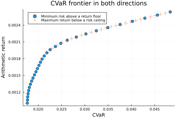
3. The MeanRisk frontier vs the NearOptimalCentering frontier
Each point of the frontier above lies at the edge of the set of feasible portfolios, because it is the exact optimum of its problem. NearOptimalCentering, NOC for short, computes a centred frontier instead. At each point it returns the portfolio at the analytic centre of the set of near-optimal portfolios, not the one at its edge. That portfolio gives up a little of the objective, holds more assets, and moves less when the prior changes. The NOC page shows how it finds the centre. Here we use it only to compute a frontier.
NOC solves a harder problem than MeanRisk, so one solver setting can fail to converge. We give it seven solvers, whose max_step_fraction falls from 0.99 to 0.7.
slv_noc = [Solver(; name = Symbol("clarabel$i"), solver = Clarabel.Optimizer, settings = Dict("verbose" => false, "max_step_fraction" => f), check_sol = (; allow_local = true, allow_almost = true)) for (i, f) in enumerate((0.99, 0.95, 0.9, 0.85, 0.8, 0.75, 0.7))]7-element Vector{Solver{Symbol, UnionAll, Dict{String, Real}, @NamedTuple{allow_local::Bool, allow_almost::Bool}, Bool}}:
Solver
name ┼ Symbol: :clarabel1
solver ┼ UnionAll: Clarabel.MOIwrapper.Optimizer
settings ┼ Dict{String, Real}: Dict{String, Real}("max_step_fraction" => 0.99, "verbose" => false)
check_sol ┼ @NamedTuple{allow_local::Bool, allow_almost::Bool}: (allow_local = true, allow_almost = true)
add_bridges ┴ Bool: true
Solver
name ┼ Symbol: :clarabel2
solver ┼ UnionAll: Clarabel.MOIwrapper.Optimizer
settings ┼ Dict{String, Real}: Dict{String, Real}("max_step_fraction" => 0.95, "verbose" => false)
check_sol ┼ @NamedTuple{allow_local::Bool, allow_almost::Bool}: (allow_local = true, allow_almost = true)
add_bridges ┴ Bool: true
Solver
name ┼ Symbol: :clarabel3
solver ┼ UnionAll: Clarabel.MOIwrapper.Optimizer
settings ┼ Dict{String, Real}: Dict{String, Real}("max_step_fraction" => 0.9, "verbose" => false)
check_sol ┼ @NamedTuple{allow_local::Bool, allow_almost::Bool}: (allow_local = true, allow_almost = true)
add_bridges ┴ Bool: true
Solver
name ┼ Symbol: :clarabel4
solver ┼ UnionAll: Clarabel.MOIwrapper.Optimizer
settings ┼ Dict{String, Real}: Dict{String, Real}("max_step_fraction" => 0.85, "verbose" => false)
check_sol ┼ @NamedTuple{allow_local::Bool, allow_almost::Bool}: (allow_local = true, allow_almost = true)
add_bridges ┴ Bool: true
Solver
name ┼ Symbol: :clarabel5
solver ┼ UnionAll: Clarabel.MOIwrapper.Optimizer
settings ┼ Dict{String, Real}: Dict{String, Real}("max_step_fraction" => 0.8, "verbose" => false)
check_sol ┼ @NamedTuple{allow_local::Bool, allow_almost::Bool}: (allow_local = true, allow_almost = true)
add_bridges ┴ Bool: true
Solver
name ┼ Symbol: :clarabel6
solver ┼ UnionAll: Clarabel.MOIwrapper.Optimizer
settings ┼ Dict{String, Real}: Dict{String, Real}("max_step_fraction" => 0.75, "verbose" => false)
check_sol ┼ @NamedTuple{allow_local::Bool, allow_almost::Bool}: (allow_local = true, allow_almost = true)
add_bridges ┴ Bool: true
Solver
name ┼ Symbol: :clarabel7
solver ┼ UnionAll: Clarabel.MOIwrapper.Optimizer
settings ┼ Dict{String, Real}: Dict{String, Real}("max_step_fraction" => 0.7, "verbose" => false)
check_sol ┼ @NamedTuple{allow_local::Bool, allow_almost::Bool}: (allow_local = true, allow_almost = true)
add_bridges ┴ Bool: true
We build both frontiers with the same return floor, a Frontier of 15 points, so that only the optimiser differs.
ret15 = ArithmeticReturn(; settings = JuMPReturnsSettings(; lb = Frontier(; N = 15)))resM = optimise(MeanRisk(; opt = JuMPOptimiser(; pe = pr, slv = slv_noc, ret = ret15), r = r))resN = optimise(NearOptimalCentering(; opt = JuMPOptimiser(; pe = pr, slv = slv_noc, ret = ret15), r = r))NearOptimalCenteringResult
jr ┼ JuMPOptimisationResult
│ pa ┼ ProcessedJuMPOptimiserAttributes
│ │ pr ┼ LowOrderPrior
│ │ │ X ┼ 252×20 Matrix{Float64}
│ │ │ o_X ┼ nothing
│ │ │ mu ┼ 20-element Vector{Float64}
│ │ │ sigma ┼ 20×20 Matrix{Float64}
│ │ │ chol ┼ nothing
│ │ │ w ┼ nothing
│ │ │ ens ┼ nothing
│ │ │ kld ┼ nothing
│ │ │ ow ┼ nothing
│ │ │ rr ┼ nothing
│ │ │ fpr ┼ nothing
│ │ │ x_src ┼ nothing
│ │ │ ss_gaps ┼ nothing
│ │ │ pc ┴ nothing
│ │ wb ┼ WeightBounds
│ │ │ lb ┼ 20-element StepRangeLen{Float64, Base.TwicePrecision{Float64}, Base.TwicePrecision{Float64}, Int64}
│ │ │ ub ┴ 20-element StepRangeLen{Float64, Base.TwicePrecision{Float64}, Base.TwicePrecision{Float64}, Int64}
│ │ lt ┼ nothing
│ │ st ┼ nothing
│ │ lcsr ┼ nothing
│ │ ctr ┼ nothing
│ │ gcardr ┼ nothing
│ │ sgcardr ┼ nothing
│ │ smtx ┼ nothing
│ │ sgmtx ┼ nothing
│ │ slt ┼ nothing
│ │ sst ┼ nothing
│ │ sglt ┼ nothing
│ │ sgst ┼ nothing
│ │ tn ┼ nothing
│ │ fees ┼ nothing
│ │ plr ┼ nothing
│ │ ret ┼ ArithmeticReturn
│ │ │ settings ┼ JuMPReturnsSettings
│ │ │ │ scale ┼ Float64: 1.0
│ │ │ │ lb ┼ Frontier
│ │ │ │ │ N ┼ Int64: 15
│ │ │ │ │ factor ┼ Int64: 1
│ │ │ │ │ bound ┴ LinearBound()
│ │ │ │ rte ┼ Bool: true
│ │ │ │ fee ┼ Bool: true
│ │ │ │ mic ┴ Bool: true
│ │ │ ucs ┼ nothing
│ │ │ mu ┼ 20-element Vector{Float64}
│ │ │ mtx_sqrt ┴ EigenFallbackSquareRoot()
│ │ sca ┼ SumScalariser()
│ │ imsk ┴ nothing
│ retcode ┼ OptimisationSuccess
│ │ res ┴ nothing
│ sol ┼ 15-element Vector{JuMPOptimisationSolution}
│ │ JuMPOptimisationSolution ⋯
│ │ JuMPOptimisationSolution ⋯
│ │ JuMPOptimisationSolution ⋯
│ │ JuMPOptimisationSolution ⋯
│ │ JuMPOptimisationSolution ⋯
│ │ JuMPOptimisationSolution ⋯
│ │ JuMPOptimisationSolution ⋯
│ │ JuMPOptimisationSolution ⋯
│ │ JuMPOptimisationSolution ⋯
│ │ JuMPOptimisationSolution ⋯
│ │ JuMPOptimisationSolution ⋯
│ │ JuMPOptimisationSolution ⋯
│ │ JuMPOptimisationSolution ⋯
│ │ JuMPOptimisationSolution ⋯
│ │ JuMPOptimisationSolution ⋯
│ model ┼ A JuMP Model
│ │ ├ solver: Clarabel
│ │ ├ objective_sense: MIN_SENSE
│ │ │ └ objective_function_type: AffExpr
│ │ ├ num_variables: 317
│ │ ├ num_constraints: 300
│ │ │ ├ AffExpr in MOI.EqualTo{Float64}: 1
│ │ │ ├ Vector{AffExpr} in MOI.Nonnegatives: 2
│ │ │ ├ Vector{AffExpr} in MOI.Nonpositives: 1
│ │ │ ├ Vector{AffExpr} in MOI.ExponentialCone: 42
│ │ │ ├ VariableRef in MOI.GreaterThan{Float64}: 252
│ │ │ └ VariableRef in MOI.Parameter{Float64}: 2
│ │ └ Names registered in the model
│ │ └ :T, :X, :bgt, :ccvar_1, :clog_delta_w, :clog_ret, :clog_risk, :clog_w, :cvar_risk_1, :k, :log_delta_w, :log_ret, :log_risk, :log_w, :lw, :net_X, :noc_rk, :noc_rt, :obj_expr, :ret, :ret_1, :ret_vec, :risk, :risk_vec, :sc, :so, :var_1, :w, :w_gross_ub, :w_lb, :w_ub, :z_cvar_1
r ┼ ConditionalValueatRisk
│ settings ┼ RiskMeasureSettings
│ │ scale ┼ Float64: 1.0
│ │ ub ┼ nothing
│ │ rke ┴ Bool: true
│ alpha ┼ Float64: 0.05
│ w ┴ nothing
w_min_retcode ┼ OptimisationSuccess
│ res ┴ Dict{Any, Any}: Dict{Any, Any}()
w_opt_retcode ┼ 15-element Vector{OptimisationSuccess}
│ OptimisationSuccess ⋯
│ OptimisationSuccess ⋯
│ OptimisationSuccess ⋯
│ OptimisationSuccess ⋯
│ OptimisationSuccess ⋯
│ OptimisationSuccess ⋯
│ OptimisationSuccess ⋯
│ OptimisationSuccess ⋯
│ OptimisationSuccess ⋯
│ OptimisationSuccess ⋯
│ OptimisationSuccess ⋯
│ OptimisationSuccess ⋯
│ OptimisationSuccess ⋯
│ OptimisationSuccess ⋯
│ OptimisationSuccess ⋯
w_max_retcode ┼ OptimisationSuccess
│ res ┴ Dict{Any, Any}: Dict{Any, Any}()
noc_retcode ┼ 15-element Vector{OptimisationSuccess}
│ OptimisationSuccess ⋯
│ OptimisationSuccess ⋯
│ OptimisationSuccess ⋯
│ OptimisationSuccess ⋯
│ OptimisationSuccess ⋯
│ OptimisationSuccess ⋯
│ OptimisationSuccess ⋯
│ OptimisationSuccess ⋯
│ OptimisationSuccess ⋯
│ OptimisationSuccess ⋯
│ OptimisationSuccess ⋯
│ OptimisationSuccess ⋯
│ OptimisationSuccess ⋯
│ OptimisationSuccess ⋯
│ OptimisationSuccess ⋯
fb ┴ nothing
NOC solves many MeanRisk problems and returns one retcode for all of them. We check that it is a success.
isa(resN.retcode, OptimisationSuccess)trueWe print the largest single weight at each point of both frontiers. A lower number means that the portfolio spreads its weight over more assets. The NOC column is lower at most points. The two columns come close at the high-return end, where both frontiers approach the one portfolio that maximises the return.
maxw(ws) = [round(maximum(w) * 100; digits = 1) for w in ws]pretty_table(DataFrame("point" => 1:15, "MeanRisk max w %" => maxw(resM.w), "NOC max w %" => maxw(resN.w)); title = "Largest single weight along each frontier")Largest single weight along each frontier
┌───────┬──────────────────┬─────────────┐
│ point │ MeanRisk max w % │ NOC max w % │
│ Int64 │ Float64 │ Float64 │
├───────┼──────────────────┼─────────────┤
│ 1 │ 45.3 │ 35.3 │
│ 2 │ 37.2 │ 34.5 │
│ 3 │ 34.5 │ 41.1 │
│ 4 │ 40.1 │ 43.2 │
│ 5 │ 46.9 │ 44.8 │
│ 6 │ 52.9 │ 45.2 │
│ 7 │ 59.0 │ 46.3 │
│ 8 │ 65.6 │ 46.5 │
│ 9 │ 71.6 │ 44.0 │
│ 10 │ 60.2 │ 46.1 │
│ 11 │ 51.9 │ 54.8 │
│ 12 │ 63.9 │ 65.8 │
│ 13 │ 75.9 │ 77.2 │
│ 14 │ 88.0 │ 87.6 │
│ 15 │ 100.0 │ 93.6 │
└───────┴──────────────────┴─────────────┘We plot both frontiers with the CVaR on the x-axis and the return on the y-axis. The NOC frontier lies inside the MeanRisk frontier, to its right, because for a given return it takes a little more CVaR. That extra CVaR is the cost of a portfolio at the centre of the near-optimal set instead of at its edge.
xs_M = [expected_risk(rcvar, w, pr.X) for w in resM.w]ys_M = [expected_return(ArithmeticReturn(), w, pr) for w in resM.w]xs_N = [expected_risk(rcvar, w, pr.X) for w in resN.w]ys_N = [expected_return(ArithmeticReturn(), w, pr) for w in resN.w]plot(xs_M, ys_M; seriestype = :scatter, marker = (:circle, 5), label = "MeanRisk (edge)", xlabel = "CVaR", ylabel = "Arithmetic return", title = "MeanRisk and NOC frontiers")plot!(xs_N, ys_N; seriestype = :scatter, marker = (:diamond, 6), label = "NOC (centred)")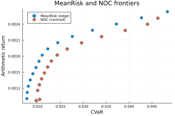
The stacked areas show the weights at each point of the MeanRisk frontier.
plot_stacked_area_composition(resM.w, rd.nx)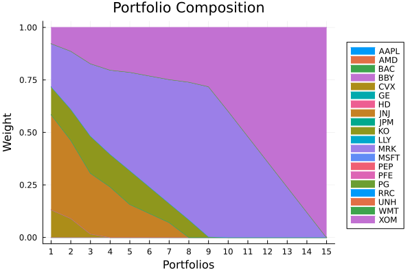
The MeanRisk frontier holds a few assets at its low-risk end and one at its high-return end. Compare the number of coloured bands at each end with the same plot for the NOC frontier below.
plot_stacked_area_composition(resN.w, rd.nx)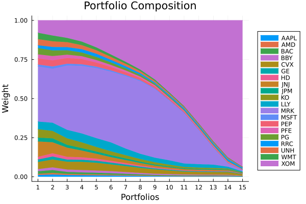
4. Visualising the frontier
The efficient frontier is a special case of a Pareto front, and plot_measures plots one on any pair of axes. Keywords set the measure on the x-axis, the y-axis, the z-axis and the colour bar. Here the CVaR is on the x-axis, the arithmetic return on the y-axis, and the colour shows the risk-return ratio.
plot_measures(resA.w, resA.pr; x = r, y = ExpectedReturn(; rt = resA.ret), c = ExpectedReturnRiskRatio(; rt = resA.ret, rk = r, rf = rf), title = "Efficient frontier", xlabel = "CVaR", ylabel = "Arithmetic Return", colorbar_title = "\nReturn/Risk Ratio", right_margin = 6Plots.mm)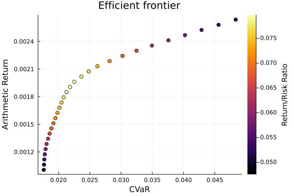
plot_measures takes any pair of measures, so you can view the same 30 portfolios on other axes. Here the y-axis is the conditional drawdown at risk (CDaR), ConditionalDrawdownatRisk, which is the CVaR of the drawdowns. The colour is the ratio of the CDaR to the CVaR. These portfolios do not minimise the CDaR, so this plot is not a front of the CVaR against the CDaR.
plot_measures(resA.w, resA.pr; x = r, y = ConditionalDrawdownatRisk(), c = RiskRatio(; r1 = ConditionalDrawdownatRisk(), r2 = r), title = "CDaR of the CVaR frontier", xlabel = "CVaR", ylabel = "CDaR", colorbar_title = "\nCDaR/CVaR Ratio", right_margin = 6Plots.mm)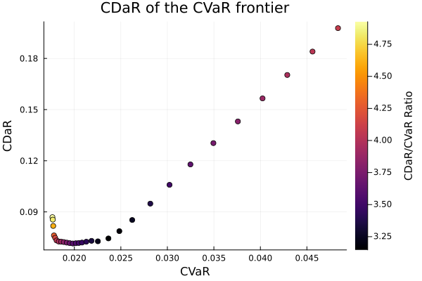
This page was generated using Literate.jl.