The source files can be found in examples/.
Performance attribution and post-optimisation diagnostics
An optimiser gives you weights. It does not tell you how the portfolio behaves. Before you trust an allocation, you measure what it would have done: how wealth would have grown, how deep and how long the drawdowns were, which assets the risk comes from, and how much the fees take from the return. None of these is what the portfolios below optimise. You compute them after optimise, and they take any weights: the output of an optimiser, a benchmark, a portfolio you already hold, or equal weights.
The plotting and reporting page draws plots. This page uses the functions that return the numbers and the series behind those plots, so you can put them in a table and compare them.
cumulative_returnsreturns the equity curve, simple (a sum) or compounded (a product).drawdownsreturns the loss from the running peak, from which the maximum drawdown, the average drawdown and the Ulcer index follow.calc_net_returnsandcalc_feesreturn the returns net of fees and the fees themselves, so you can see how much of the performance the fees take.risk_contributionreturns the share of the risk of the portfolio that each asset contributes.
Reach for these functions after you choose a portfolio, to compare candidates on the returns they would have made, on the concentration of their risk and on their fees, without a new optimisation. They take plain weights, so they also report on a benchmark or on a portfolio from outside the library.
using PortfolioOptimisers, PrettyTables, DataFrames, Statisticsresfmt = (v, i, j) -> begin if j == 1 return v else return isa(v, Number) ? "$(round(v * 100, digits = 3)) %" : v endend;1. Candidate portfolios
We compare three portfolios: a minimum-variance and a maximum-ratio portfolio from MeanRisk, and an equal-weight portfolio. The equal-weight portfolio is a plain vector, and every function below takes it as it takes the output of an optimiser. The sections below score each portfolio on the returns the optimiser fitted, so their numbers are in sample.
using CSV, TimeSeries, ClarabelX = TimeArray(CSV.File(joinpath(@__DIR__, "..", "SP500.csv.gz")); timestamp = :Date)[(end - 252):end]rd = prices_to_returns(X)pr = prior(EmpiricalPrior(), rd)rf = 4.2 / 100 / 252slv = Solver(; name = :clarabel, solver = Clarabel.Optimizer, settings = Dict("verbose" => false), check_sol = (; allow_local = true, allow_almost = true))w_min = optimise(MeanRisk(; obj = MinimumRisk(), opt = JuMPOptimiser(; pe = pr, slv = slv))).ww_ratio = optimise(MeanRisk(; obj = MaximumRatio(; rf = rf), opt = JuMPOptimiser(; pe = pr, slv = slv))).ww_ew = fill(inv(length(rd.nx)), length(rd.nx))books = ["Min variance" => w_min, "Max ratio" => w_ratio, "Equal weight" => w_ew]port_ret = [name => rd.X * w for (name, w) in books]3-element Vector{Pair{String, Vector{Float64}}}:
"Min variance" => [0.0026813226223467252, 0.0010718963591281865, -0.001091427248523713, 0.004544617536042419, 0.0033640670294395186, 0.010241746052436444, -0.0005334075714804237, 0.010636902007924172, 0.0020214817396439094, -0.0020684143227997407 … 0.0016026835814606367, -0.013295284199452188, -0.008357208547583001, 0.0014778555240849338, 0.0036899176302639717, 0.011666675299059192, -0.005956204640016675, 0.007175142095467477, 0.003337745419751359, -0.008845799550049428]
"Max ratio" => [-0.0017735403232562238, -0.0003663495800995623, -0.002042024455486072, 0.015047999836559611, 0.014001426877989446, 0.02024912490359903, 0.007577814646385911, 0.015092279238491976, 0.014987394169298188, 0.008706910967850243 … 0.005701709798627909, -0.014619597724759393, -0.00497424702546818, 0.0029772392002589765, 0.0065411200233170905, 0.012794339416953182, -0.00609059966693818, 0.01266787003000156, 0.006264546445565564, -0.011709263471352042]
"Equal weight" => [-7.529306018214316e-5, -0.003943468929117261, -0.000616891006106372, 0.007922868362850641, 0.0038386302710631784, -0.0068189323184242295, -0.0008574365354449756, 0.0019159331199490334, 0.002182170970507891, 0.010325853772815504 … -0.005087357906633977, -0.01666983095423833, -0.01116567508679087, -0.0026616271633638847, 0.003791176075818492, 0.016771917527164504, -0.013691693040682809, 0.00895206870792011, 0.0009859963867063877, -0.012904987269724347]2. Cumulative returns: the equity curve
cumulative_returns turns a series of returns into a path of wealth. Its second argument, compound, chooses how:
false, the default, sums the returns,cumsum(X). This is the absolute cumulative return. It adds up period by period and is easy to read over a short horizon.truemultiplies them,cumprod(1 .+ X). This is the relative, or geometric, multiple of wealth, which is what an investor who reinvests gets.
The table prints the last compounded multiple of wealth of each portfolio.
final_wealth = [name => cumulative_returns(r, true)[end] for (name, r) in port_ret]pretty_table(DataFrame(; book = first.(final_wealth), Symbol("compounded wealth (×)") => [round(last(p); digits = 4) for p in final_wealth]); title = "Final compounded wealth multiple over the sample")Final compounded wealth multiple over the sample
┌──────────────┬───────────────────────┐
│ book │ compounded wealth (×) │
│ String │ Float64 │
├──────────────┼───────────────────────┤
│ Min variance │ 1.2015 │
│ Max ratio │ 1.6234 │
│ Equal weight │ 1.0166 │
└──────────────┴───────────────────────┘3. Drawdowns
drawdowns returns the drawdown at each point, the loss from the highest value reached before it. From that series we compute three statistics: the maximum drawdown, which is the worst loss; the average drawdown, which is the mean depth over time; and the Ulcer index, the root mean square of the depth, which weighs a deep drawdown more than a shallow one. We use compounded drawdowns, to match the compounded equity curve. A drawdown is zero or negative, so we negate the minimum and the mean.
dd_stats = map(port_ret) do (name, r) dd = drawdowns(r, true) return (name = name, max_dd = -minimum(dd), avg_dd = -mean(dd), ulcer = sqrt(mean(dd .^ 2)))endpretty_table(DataFrame(dd_stats); formatters = [resfmt], title = "Drawdown statistics") Drawdown statistics
┌──────────────┬──────────┬─────────┬─────────┐
│ name │ max_dd │ avg_dd │ ulcer │
│ String │ Float64 │ Float64 │ Float64 │
├──────────────┼──────────┼─────────┼─────────┤
│ Min variance │ 9.027 % │ 2.749 % │ 3.621 % │
│ Max ratio │ 9.537 % │ 2.132 % │ 3.013 % │
│ Equal weight │ 14.712 % │ 5.118 % │ 6.369 % │
└──────────────┴──────────┴─────────┴─────────┘4. A scorecard of performance
We compute the statistics you would report for a portfolio: the annualised return and volatility, the annualised Sharpe ratio net of the risk-free rate, the maximum drawdown, and the Calmar ratio, which is the annualised return divided by the maximum drawdown. All of them come from the return series of each portfolio, with no new optimisation.
scorecard = map(port_ret) do (name, r) ann_ret = mean(r) * 252 ann_vol = std(r) * sqrt(252) sharpe = (mean(r) - rf) / std(r) * sqrt(252) max_dd = -minimum(drawdowns(r, true)) return (book = name, ann_return = ann_ret, ann_vol = ann_vol, sharpe = sharpe, max_drawdown = max_dd, calmar = ann_ret / max_dd)endpretty_table(DataFrame(scorecard); formatters = [(v, i, j) -> (if j in (2, 3, 5) "$(round(v*100, digits=2)) %" elseif isa(v, Number) round(v; digits = 3) else v end)], title = "Realised-performance scorecard") Realised-performance scorecard
┌──────────────┬────────────┬─────────┬─────────┬──────────────┬─────────┐
│ book │ ann_return │ ann_vol │ sharpe │ max_drawdown │ calmar │
│ String │ Float64 │ Float64 │ Float64 │ Float64 │ Float64 │
├──────────────┼────────────┼─────────┼─────────┼──────────────┼─────────┤
│ Min variance │ 19.46 % │ 14.83 % │ 1.028 │ 9.03 % │ 2.155 │
│ Max ratio │ 50.35 % │ 19.31 % │ 2.39 │ 9.54 % │ 5.28 │
│ Equal weight │ 3.71 % │ 20.36 % │ -0.024 │ 14.71 % │ 0.252 │
└──────────────┴────────────┴─────────┴─────────┴──────────────┴─────────┘5. Fees: gross and net returns
A portfolio with a good gross return can have a poor one after fees. calc_net_returns deducts a Fees schedule from the returns. calc_fees returns the fees as a pair: the charge on every observation, and the one-off charge on the first observation alone. calc_total_fees adds the pair up over a whole holding period.
The fees have two time bases. l, s and tn are rates per period, so calc_net_returns(w, X, fees) deducts them on every row of X. l is proportional to the long positions and s to the short ones, and tn to the turnover. Over 252 daily observations, a rate l per period adds up to about 252 * l over the year, before compounding. fl and fs are charged once for the whole holding period on each position that is not zero, and on a return series they are a fraction of capital. fees.fa decides where on the series that charge falls. We charge l = 0.0005, five basis points per period on the long positions, and compare the compounded wealth gross and net of it. The table also prints the fee of one period and the total over 252 periods.
fees = Fees(; l = 0.0005)gross_ret = rd.X * w_rationet_ret = calc_net_returns(w_ratio, rd.X, fees)single_period_fee, _ = calc_fees(w_ratio, size(rd.X, 1), fees)pretty_table(DataFrame(; quantity = ["Gross compounded wealth (×)", "Net compounded wealth (×)", "Single-period fee (fraction)", "Total fee over 252 periods"], value = [round(cumulative_returns(gross_ret, true)[end]; digits = 4), round(cumulative_returns(net_ret, true)[end]; digits = 4), round(single_period_fee; digits = 5), round(calc_total_fees(w_ratio, 252, fees); digits = 4)]); title = "Wealth and fees of the maximum-ratio portfolio, 5 basis points per period on the long positions")Wealth and fees of the maximum-ratio portfolio, 5 basis points per period on the long positions
┌──────────────────────────────┬─────────┐
│ quantity │ value │
│ String │ Float64 │
├──────────────────────────────┼─────────┤
│ Gross compounded wealth (×) │ 1.6234 │
│ Net compounded wealth (×) │ 1.4315 │
│ Single-period fee (fraction) │ 0.0005 │
│ Total fee over 252 periods │ 0.126 │
└──────────────────────────────┴─────────┘6. Risk attribution
risk_contribution splits the total risk into the share of each asset. As with the plots, a quadratic risk measure needs the covariance of the data, so pass factory(Variance(), pr), not a bare Variance(). We scale the contributions to sum to one, and the table prints the eight largest of the minimum-variance portfolio beside their weights.
rc = risk_contribution(factory(Variance(), pr), w_min, rd.X)rc ./= sum(rc)rc_df = sort(DataFrame(; asset = rd.nx, weight = w_min, risk_share = rc), :risk_share; rev = true)pretty_table(first(rc_df, 8); formatters = [resfmt], title = "The eight largest risk shares in the minimum-variance portfolio")The eight largest risk shares in the minimum-variance portfolio
┌────────┬──────────┬────────────┐
│ asset │ weight │ risk_share │
│ String │ Float64 │ Float64 │
├────────┼──────────┼────────────┤
│ JNJ │ 36.974 % │ 36.972 % │
│ MRK │ 17.467 % │ 17.467 % │
│ KO │ 11.161 % │ 11.163 % │
│ WMT │ 9.355 % │ 9.355 % │
│ PEP │ 8.978 % │ 8.978 % │
│ CVX │ 7.432 % │ 7.434 % │
│ XOM │ 4.725 % │ 4.725 % │
│ PG │ 2.353 % │ 2.352 % │
└────────┴──────────┴────────────┘On the minimum-variance portfolio the two columns match. At the minimum of the variance, a small move of weight between two assets in the portfolio does not change the variance, so each of its assets adds the same variance per unit of weight. The share of the risk of each asset is then its weight. We compute the same shares for the maximum-ratio portfolio, and the table prints the assets with a weight above 0.01 %.
rc_ratio = risk_contribution(factory(Variance(), pr), w_ratio, rd.X)rc_ratio ./= sum(rc_ratio)rc_ratio_df = sort(DataFrame(; asset = rd.nx, weight = w_ratio, risk_share = rc_ratio), :risk_share; rev = true)pretty_table(filter(:weight => >(1e-4), rc_ratio_df); formatters = [resfmt], title = "Weight and risk share of each asset of the maximum-ratio portfolio with a weight above 0.01 %")Weight and risk share of each asset of the maximum-ratio portfolio with a weight above 0.01 %
┌────────┬──────────┬────────────┐
│ asset │ weight │ risk_share │
│ String │ Float64 │ Float64 │
├────────┼──────────┼────────────┤
│ MRK │ 65.977 % │ 54.072 % │
│ XOM │ 34.02 % │ 45.926 % │
└────────┴──────────┴────────────┘Here the two columns differ, and XOM takes a larger share of the risk than of the weight. An asset with a high volatility, or a high correlation with the other assets, can contribute more risk than its weight, and the weights alone do not show it.
7. The equity curves
The last plot draws the compounded wealth of the three portfolios over the sample.
using StatsPlots, GraphRecipescurves = [name => cumulative_returns(r, true) for (name, r) in port_ret]plot(cumulative_returns(port_ret[1][2], true); label = first(port_ret[1]), xlabel = "Day", ylabel = "Compounded wealth (×)", title = "Realised equity curves", legend = :topleft)for (name, r) in port_ret[2:end] plot!(cumulative_returns(r, true); label = name)endcurrent()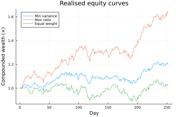
Summary
On this sample the three portfolios differ as follows:
- The maximum-ratio portfolio ends with the largest compounded wealth of the three, and the equal-weight portfolio has the largest value of all three drawdown statistics.
- A fee of five basis points per period on the long positions lowers the compounded wealth of the maximum-ratio portfolio, and
calc_total_feesgives the fee over the whole sample. - On the minimum-variance portfolio the share of the risk of each asset equals its weight. On the maximum-ratio portfolio the two differ.
This page was generated using Literate.jl.