The source files can be found in examples/.
Custom objectives and constraints
Each keyword of the JuMPOptimiser, such as the bounds, the budgets, turnover, fees and cardinality, adds a ready-made part to the problem. When a mandate needs something that no keyword covers, you can write a term into the JuMP model yourself, in one of two ways.
- Subtype
CustomJuMPObjective, pass it to thecobjkeyword, and write a method ofadd_custom_objective_term!. The term puts a price on a preference in the objective. - Subtype
CustomJuMPConstraint, pass it to theccntkeyword, and write a method ofadd_custom_constraint!. The constraint must hold in the solution.
Each keyword takes one estimator or a vector of them. The library calls the function with your estimator as an argument, so Julia picks your method by the type of the estimator. A custom term is a struct that holds its data, and one method. If you subtype one of the two types and write no method, the optimisation throws an error that names the missing method. This page builds both kinds of term, shows the two rules that keep a constraint correct, and combines several terms in one problem. The constraints and costs guide gives a short summary of the same features.
Reach for a custom term when your preference is a number per asset that no group string can express, such as a factor score, a carbon intensity or a liquidity penalty. Reach for it also for a relation between weights that is not a plain linear bound. If a linear or group constraint (lcse) or another keyword can express it, use that instead, because the library tests those and they work with every other keyword. Write a custom term only when no keyword fits.
using PortfolioOptimisers, CSV, TimeSeries, DataFrames, PrettyTables, Clarabel, StatsPlots, GraphRecipesusing JuMP: JuMPresfmt = (v, i, j) -> begin return if j == 1 v else isa(v, AbstractFloat) ? "$(round(v*100, digits=3)) %" : v endend;1. Data and a momentum score
We fit one empirical prior, set up one solver, and optimise a minimum risk baseline, so you can compare every custom term with the same portfolio. The preference is a momentum score, the sum of each asset's daily returns over the last 63 days, standardised across the assets. It is a number per asset, which is the case that custom terms are for.
X = TimeArray(CSV.File(joinpath(@__DIR__, "..", "SP500.csv.gz")); timestamp = :Date)[(end - 252):end]rd = prices_to_returns(X)pr = prior(EmpiricalPrior(), rd)slv = Solver(; name = :clarabel, solver = Clarabel.Optimizer, settings = Dict("verbose" => false), check_sol = (; allow_local = true, allow_almost = true))rf = 4.2 / 100 / 252score = let m = vec(sum(rd.X[(end - 62):end, :]; dims = 1)) (m .- mean(m)) ./ std(m)endres_base = optimise(MeanRisk(; obj = MinimumRisk(), opt = JuMPOptimiser(; pe = pr, slv = slv)))MeanRiskResult
jr ┼ JuMPOptimisationResult
│ pa ┼ ProcessedJuMPOptimiserAttributes
│ │ pr ┼ LowOrderPrior
│ │ │ X ┼ 252×20 Matrix{Float64}
│ │ │ o_X ┼ nothing
│ │ │ mu ┼ 20-element Vector{Float64}
│ │ │ sigma ┼ 20×20 Matrix{Float64}
│ │ │ chol ┼ nothing
│ │ │ w ┼ nothing
│ │ │ ens ┼ nothing
│ │ │ kld ┼ nothing
│ │ │ ow ┼ nothing
│ │ │ rr ┼ nothing
│ │ │ fpr ┴ nothing
│ │ wb ┼ WeightBounds
│ │ │ lb ┼ 20-element StepRangeLen{Float64, Base.TwicePrecision{Float64}, Base.TwicePrecision{Float64}, Int64}
│ │ │ ub ┴ 20-element StepRangeLen{Float64, Base.TwicePrecision{Float64}, Base.TwicePrecision{Float64}, Int64}
│ │ lt ┼ nothing
│ │ st ┼ nothing
│ │ lcsr ┼ nothing
│ │ ctr ┼ nothing
│ │ gcardr ┼ nothing
│ │ sgcardr ┼ nothing
│ │ smtx ┼ nothing
│ │ sgmtx ┼ nothing
│ │ slt ┼ nothing
│ │ sst ┼ nothing
│ │ sglt ┼ nothing
│ │ sgst ┼ nothing
│ │ tn ┼ nothing
│ │ fees ┼ nothing
│ │ plr ┼ nothing
│ │ ret ┼ ArithmeticReturn
│ │ │ settings ┼ JuMPReturnsSettings
│ │ │ │ scale ┼ Float64: 1.0
│ │ │ │ lb ┼ nothing
│ │ │ │ rte ┼ Bool: true
│ │ │ │ fee ┼ Bool: true
│ │ │ │ mic ┴ Bool: true
│ │ │ ucs ┼ nothing
│ │ │ mu ┴ 20-element Vector{Float64}
│ │ sca ┼ SumScalariser()
│ │ imsk ┴ nothing
│ retcode ┼ OptimisationSuccess
│ │ res ┴ Dict{Any, Any}: Dict{Any, Any}()
│ sol ┼ JuMPOptimisationSolution
│ │ w ┴ 20-element Vector{Float64}
│ model ┼ A JuMP Model
│ │ ├ solver: Clarabel
│ │ ├ objective_sense: MIN_SENSE
│ │ │ └ objective_function_type: QuadExpr
│ │ ├ num_variables: 21
│ │ ├ num_constraints: 4
│ │ │ ├ AffExpr in MOI.EqualTo{Float64}: 1
│ │ │ ├ Vector{AffExpr} in MOI.Nonnegatives: 1
│ │ │ ├ Vector{AffExpr} in MOI.Nonpositives: 1
│ │ │ └ Vector{AffExpr} in MOI.SecondOrderCone: 1
│ │ └ Names registered in the model
│ │ └ :G, :T, :bgt, :cdev_soc_1, :dev_1, :k, :lw, :obj_expr, :ret, :ret_1, :ret_vec, :risk, :risk_minimised, :risk_vec, :sc, :so, :variance_flag, :variance_risk_1, :w, :w_gross_ub, :w_lb, :w_ub
r ┼ Variance
│ settings ┼ RiskMeasureSettings
│ │ scale ┼ Float64: 1.0
│ │ ub ┼ nothing
│ │ rke ┴ Bool: true
│ sigma ┼ 20×20 Matrix{Float64}
│ chol ┼ nothing
│ rc ┼ nothing
│ alg ┴ SquaredSOCRiskExpr()
fb ┴ nothing
The momentum exposure of a portfolio is score' * w. The minimum risk baseline takes no account of momentum. We print its exposure. Then we raise the exposure, first with a term in the objective and then with a constraint.
base_exposure = score' * res_base.w0.204210918363751272. A custom objective: a tilt toward momentum
The library calls your method of add_custom_objective_term! while it builds the model. The method adds a term to the objective penalty, a sum of terms that the library adds to the objective. Its signature is
add_custom_objective_term!(model, obj, cobj, optimiser, attrs)modelis theJuMPmodel that the library builds.objis theObjectiveFunctionof the problem, such asMinimumRiskorMaximumUtility. Dispatch on it if your term must change with the objective. You do not need it to get the sign right.cobjis your estimator, and your method dispatches on its type.optimiseris the optimisation estimator, for example theMeanRiskitself. Itsoptfield is theJuMPOptimiser.attrsis aProcessedJuMPOptimiserAttributes, the data of the problem after processing. It holds the prior inattrs.pr, the returns estimator inattrs.ret, the weight bounds inattrs.wb, and more. Read it if your term computes its numbers from the data.
Get the weight variables with get_w, not with model[:w]. If the model has no weight variables yet, get_w throws an error that says so.
Add the term with add_to_objective_penalty!, not by a change to the objective expression. Then the term is correct under every objective.
Some objectives are minimised and some are maximised, and MaximumRatio can be either, depending on the risk measure. A term that you add to the objective expression yourself therefore has no sign that is right in every case. The library adds the objective penalty to the objective with a factor of 1 when it minimises and -1 when it maximises. With this factor, a positive term always makes the objective worse, and a reward is a negative term. Write -λ * something_good once, and it is a reward under every objective.
The objective penalty also becomes quadratic when you add a quadratic term, such as an L2 tilt or a tracking penalty. A quadratic term therefore works with every objective, including the linear ones, where a direct change to the objective expression throws a MethodError.
struct MomentumTilt{T1, T2} <: PortfolioOptimisers.CustomJuMPObjective score::T1 lambda::T2endfunction PortfolioOptimisers.add_custom_objective_term!(model::JuMP.Model, obj, cobj::MomentumTilt, optimiser, attrs) w = PortfolioOptimisers.get_w(model) PortfolioOptimisers.add_to_objective_penalty!(model, -cobj.lambda * (cobj.score' * w)) return nothingendlambda is the price of momentum against risk. We solve for four values of lambda, and print the momentum exposure and the largest weight of each result. The smallest price above zero, 1e-4, already moves the weights far from the baseline. Each larger price raises the exposure by less than the one before, because the weights move toward the one asset with the highest score.
lambdas = [0.0, 1e-4, 5e-4, 2e-3]tilt_res = [optimise(MeanRisk(; obj = MinimumRisk(), opt = JuMPOptimiser(; pe = pr, slv = slv, cobj = MomentumTilt(score, l)))) for l in lambdas]pretty_table(DataFrame("λ (momentum price)" => lambdas, "Momentum exposure" => [score' * r.w for r in tilt_res], "Max weight" => [maximum(r.w) for r in tilt_res]); formatters = [resfmt], title = "Momentum exposure and largest weight at each λ") Momentum exposure and largest weight at each λ
┌────────────────────┬───────────────────┬────────────┐
│ λ (momentum price) │ Momentum exposure │ Max weight │
│ Float64 │ Float64 │ Float64 │
├────────────────────┼───────────────────┼────────────┤
│ 0.0 │ 20.421 % │ 36.974 % │
│ 0.0001 │ 129.535 % │ 69.305 % │
│ 0.0005 │ 139.637 % │ 83.008 % │
│ 0.002 │ 139.873 % │ 88.846 % │
└────────────────────┴───────────────────┴────────────┘The term is homogeneous of degree one in w. If you multiply the weights by a number, the term is multiplied by the same number, as the expected return is. The term stays correct when a ratio objective rescales the weights. A constraint needs more care with that rescaling, which section 5 shows.
3. The same term in a maximisation
MaximumUtility is a maximisation, where the problem above is a minimisation. We use the same MomentumTilt with no change, and print the momentum exposure without it and with it. The library adds the objective penalty with the factor of a maximisation, so the tilt is a reward here too.
util_base = optimise(MeanRisk(; obj = MaximumUtility(), opt = JuMPOptimiser(; pe = pr, slv = slv)))util_tilt = optimise(MeanRisk(; obj = MaximumUtility(), opt = JuMPOptimiser(; pe = pr, slv = slv, cobj = MomentumTilt(score, 5e-3))))util_exposures = (base = score' * util_base.w, tilted = score' * util_tilt.w)(base = 1.156107153804669, tilted = 1.4032396336091977)The library solves the maximum-ratio problem with a change of variables. Depending on the risk measure, the result is a maximisation, or a minimisation of the risk. Each form adds the objective penalty with its own factor, so the tilt is a reward in both. This fixes the sign, not the scale. A term that is not homogeneous of degree one in w still needs the variable k of section 5.
4. A custom constraint: a floor on momentum
The library calls your method of add_custom_constraint! in the same way. Its signature is
add_custom_constraint!(model, ccnt, optimiser, attrs)The arguments are those of add_custom_objective_term! without obj. ccnt is your estimator, and your method dispatches on its type.
Follow two rules when you write a constraint.
- Multiply the constraint by
get_constraint_scale, which returnsmodel[:sc]. The library scales every constraint it makes by this number, so yours then has the same scale. - Multiply each constant bound by
get_k, which returnsmodel[:k]. For most objectiveskis the constant 1, and the product changes nothing. Under a ratio objectivekis a variable at or above zero, and the solver works with rescaled weights,w_real = w / k. A constant with nokis then compared with the rescaled weights, which is the wrong comparison. Section 5 shows the result.
struct MomentumFloor{T1, T2} <: PortfolioOptimisers.CustomJuMPConstraint score::T1 floor::T2endfunction PortfolioOptimisers.add_custom_constraint!(model::JuMP.Model, ccnt::MomentumFloor, optimiser, attrs) w = PortfolioOptimisers.get_w(model) k = PortfolioOptimisers.get_k(model) sc = PortfolioOptimisers.get_constraint_scale(model) JuMP.@constraint(model, sc * (ccnt.score' * w - ccnt.floor * k) >= 0) return nothingendA floor acts differently from the tilt. When the floor binds, the exposure equals the floor, and the weights minimise the risk under that condition. A floor below the exposure of the baseline does not bind. We solve for four floors, and print the exposure of each result next to its floor. The Binds? column is yes when the exposure is at most 1e-6 above the floor.
floors = [0.0, 0.5, 1.0, 1.35]floor_res = [optimise(MeanRisk(; obj = MinimumRisk(), opt = JuMPOptimiser(; pe = pr, slv = slv, ccnt = MomentumFloor(score, f)))) for f in floors]pretty_table(DataFrame("Momentum floor" => floors, "Momentum exposure" => [score' * r.w for r in floor_res], "Binds?" => [score' * r.w > f + 1e-6 ? "no" : "yes" for (f, r) in zip(floors, floor_res)]); formatters = [resfmt], title = "Momentum floors and the exposure of the minimum-risk portfolio")Momentum floors and the exposure of the minimum-risk portfolio
┌────────────────┬───────────────────┬────────┐
│ Momentum floor │ Momentum exposure │ Binds? │
│ Float64 │ Float64 │ String │
├────────────────┼───────────────────┼────────┤
│ 0.0 │ 20.436 % │ no │
│ 0.5 │ 50.0 % │ no │
│ 1.0 │ 100.0 % │ yes │
│ 1.35 │ 135.0 % │ yes │
└────────────────┴───────────────────┴────────┘5. Why a constant bound needs k
We write the same floor without the * k. Under MinimumRisk, k is 1, so the mistake has no effect there and is easy to miss.
struct MomentumFloorNoK{T1, T2} <: PortfolioOptimisers.CustomJuMPConstraint score::T1 floor::T2endfunction PortfolioOptimisers.add_custom_constraint!(model::JuMP.Model, ccnt::MomentumFloorNoK, opt, attrs) w = PortfolioOptimisers.get_w(model) sc = PortfolioOptimisers.get_constraint_scale(model) #! This bound leaves out `* k` on purpose, to show the mistake. JuMP.@constraint(model, sc * (ccnt.score' * w - ccnt.floor) >= 0) return nothingendUnder MaximumRatio, k is a variable of the problem, so the two floors give different results. The floor with k holds the exposure of the final weights at the bound. The floor without k holds the exposure of the rescaled weights at the bound, which is a different number. We compare the two over three floors. At floor = 1.38, the version without k gives an exposure below the floor, and no error tells you.
k_floors = [1.30, 1.35, 1.38]k_compare = [(f, score' * optimise(MeanRisk(; obj = MaximumRatio(; rf = rf), opt = JuMPOptimiser(; pe = pr, slv = slv, ccnt = MomentumFloor(score, f)))).w, score' * optimise(MeanRisk(; obj = MaximumRatio(; rf = rf), opt = JuMPOptimiser(; pe = pr, slv = slv, ccnt = MomentumFloorNoK(score, f)))).w) for f in k_floors]pretty_table(DataFrame("Requested floor" => first.(k_compare), "With * k (correct)" => getindex.(k_compare, 2), "Without * k (wrong)" => getindex.(k_compare, 3)); formatters = [resfmt], title = "MaximumRatio momentum exposure, floor with and without * k") MaximumRatio momentum exposure, floor with and without * k
┌─────────────────┬────────────────────┬─────────────────────┐
│ Requested floor │ With * k (correct) │ Without * k (wrong) │
│ Float64 │ Float64 │ Float64 │
├─────────────────┼────────────────────┼─────────────────────┤
│ 1.3 │ 130.0 % │ 136.853 % │
│ 1.35 │ 135.0 % │ 136.933 % │
│ 1.38 │ 138.0 % │ 136.983 % │
└─────────────────┴────────────────────┴─────────────────────┘6. Composing several custom pieces
Both keywords take a vector of estimators, and the library applies them in order, with one method call for each. You can combine custom terms without one struct for all of them.
First, a band from two constraints. A cap is the floor with the inequality reversed, and a floor and a cap together keep the exposure inside a band. We define the cap, then give both constraints to one optimiser.
struct MomentumCap{T1, T2} <: PortfolioOptimisers.CustomJuMPConstraint score::T1 cap::T2endfunction PortfolioOptimisers.add_custom_constraint!(model::JuMP.Model, ccnt::MomentumCap, optimiser, attrs) w = PortfolioOptimisers.get_w(model) k = PortfolioOptimisers.get_k(model) sc = PortfolioOptimisers.get_constraint_scale(model) JuMP.@constraint(model, sc * (ccnt.cap * k - ccnt.score' * w) >= 0) return nothingendband = optimise(MeanRisk(; obj = MinimumRisk(), opt = JuMPOptimiser(; pe = pr, slv = slv, ccnt = [MomentumFloor(score, 0.5), MomentumCap(score, 0.8)])))MeanRiskResult
jr ┼ JuMPOptimisationResult
│ pa ┼ ProcessedJuMPOptimiserAttributes
│ │ pr ┼ LowOrderPrior
│ │ │ X ┼ 252×20 Matrix{Float64}
│ │ │ o_X ┼ nothing
│ │ │ mu ┼ 20-element Vector{Float64}
│ │ │ sigma ┼ 20×20 Matrix{Float64}
│ │ │ chol ┼ nothing
│ │ │ w ┼ nothing
│ │ │ ens ┼ nothing
│ │ │ kld ┼ nothing
│ │ │ ow ┼ nothing
│ │ │ rr ┼ nothing
│ │ │ fpr ┴ nothing
│ │ wb ┼ WeightBounds
│ │ │ lb ┼ 20-element StepRangeLen{Float64, Base.TwicePrecision{Float64}, Base.TwicePrecision{Float64}, Int64}
│ │ │ ub ┴ 20-element StepRangeLen{Float64, Base.TwicePrecision{Float64}, Base.TwicePrecision{Float64}, Int64}
│ │ lt ┼ nothing
│ │ st ┼ nothing
│ │ lcsr ┼ nothing
│ │ ctr ┼ nothing
│ │ gcardr ┼ nothing
│ │ sgcardr ┼ nothing
│ │ smtx ┼ nothing
│ │ sgmtx ┼ nothing
│ │ slt ┼ nothing
│ │ sst ┼ nothing
│ │ sglt ┼ nothing
│ │ sgst ┼ nothing
│ │ tn ┼ nothing
│ │ fees ┼ nothing
│ │ plr ┼ nothing
│ │ ret ┼ ArithmeticReturn
│ │ │ settings ┼ JuMPReturnsSettings
│ │ │ │ scale ┼ Float64: 1.0
│ │ │ │ lb ┼ nothing
│ │ │ │ rte ┼ Bool: true
│ │ │ │ fee ┼ Bool: true
│ │ │ │ mic ┴ Bool: true
│ │ │ ucs ┼ nothing
│ │ │ mu ┴ 20-element Vector{Float64}
│ │ sca ┼ SumScalariser()
│ │ imsk ┴ nothing
│ retcode ┼ OptimisationSuccess
│ │ res ┴ Dict{Any, Any}: Dict{Any, Any}()
│ sol ┼ JuMPOptimisationSolution
│ │ w ┴ 20-element Vector{Float64}
│ model ┼ A JuMP Model
│ │ ├ solver: Clarabel
│ │ ├ objective_sense: MIN_SENSE
│ │ │ └ objective_function_type: QuadExpr
│ │ ├ num_variables: 21
│ │ ├ num_constraints: 6
│ │ │ ├ AffExpr in MOI.EqualTo{Float64}: 1
│ │ │ ├ AffExpr in MOI.GreaterThan{Float64}: 2
│ │ │ ├ Vector{AffExpr} in MOI.Nonnegatives: 1
│ │ │ ├ Vector{AffExpr} in MOI.Nonpositives: 1
│ │ │ └ Vector{AffExpr} in MOI.SecondOrderCone: 1
│ │ └ Names registered in the model
│ │ └ :G, :T, :bgt, :cdev_soc_1, :dev_1, :k, :lw, :obj_expr, :ret, :ret_1, :ret_vec, :risk, :risk_minimised, :risk_vec, :sc, :so, :variance_flag, :variance_risk_1, :w, :w_gross_ub, :w_lb, :w_ub
r ┼ Variance
│ settings ┼ RiskMeasureSettings
│ │ scale ┼ Float64: 1.0
│ │ ub ┼ nothing
│ │ rke ┴ Bool: true
│ sigma ┼ 20×20 Matrix{Float64}
│ chol ┼ nothing
│ rc ┼ nothing
│ alg ┴ SquaredSOCRiskExpr()
fb ┴ nothing
Second, two objective terms. Each term of a cobj vector adds to the same objective penalty, so two tilts of 1e-4 act as one tilt of 2e-4. We solve both, and print the three exposures.
two_tilts = optimise(MeanRisk(; obj = MinimumRisk(), opt = JuMPOptimiser(; pe = pr, slv = slv, cobj = [MomentumTilt(score, 1e-4), MomentumTilt(score, 1e-4)])))one_double = optimise(MeanRisk(; obj = MinimumRisk(), opt = JuMPOptimiser(; pe = pr, slv = slv, cobj = MomentumTilt(score, 2e-4))))composition = (band = score' * band.w, two_1e4_tilts = score' * two_tilts.w, one_2e4_tilt = score' * one_double.w)(band = 0.5000014186440696, two_1e4_tilts = 1.3694760110198174, one_2e4_tilt = 1.3694760110198174)Compare the exposure of the band portfolio with [0.5, 0.8]. Then compare the exposure of the two tilts of 1e-4 with that of the one tilt of 2e-4.
Last, an objective term and a constraint together. We give a tilt to cobj and a floor to ccnt of one optimiser.
res_both = optimise(MeanRisk(; obj = MinimumRisk(), opt = JuMPOptimiser(; pe = pr, slv = slv, cobj = MomentumTilt(score, 1e-4), ccnt = MomentumFloor(score, 1.0))))MeanRiskResult
jr ┼ JuMPOptimisationResult
│ pa ┼ ProcessedJuMPOptimiserAttributes
│ │ pr ┼ LowOrderPrior
│ │ │ X ┼ 252×20 Matrix{Float64}
│ │ │ o_X ┼ nothing
│ │ │ mu ┼ 20-element Vector{Float64}
│ │ │ sigma ┼ 20×20 Matrix{Float64}
│ │ │ chol ┼ nothing
│ │ │ w ┼ nothing
│ │ │ ens ┼ nothing
│ │ │ kld ┼ nothing
│ │ │ ow ┼ nothing
│ │ │ rr ┼ nothing
│ │ │ fpr ┴ nothing
│ │ wb ┼ WeightBounds
│ │ │ lb ┼ 20-element StepRangeLen{Float64, Base.TwicePrecision{Float64}, Base.TwicePrecision{Float64}, Int64}
│ │ │ ub ┴ 20-element StepRangeLen{Float64, Base.TwicePrecision{Float64}, Base.TwicePrecision{Float64}, Int64}
│ │ lt ┼ nothing
│ │ st ┼ nothing
│ │ lcsr ┼ nothing
│ │ ctr ┼ nothing
│ │ gcardr ┼ nothing
│ │ sgcardr ┼ nothing
│ │ smtx ┼ nothing
│ │ sgmtx ┼ nothing
│ │ slt ┼ nothing
│ │ sst ┼ nothing
│ │ sglt ┼ nothing
│ │ sgst ┼ nothing
│ │ tn ┼ nothing
│ │ fees ┼ nothing
│ │ plr ┼ nothing
│ │ ret ┼ ArithmeticReturn
│ │ │ settings ┼ JuMPReturnsSettings
│ │ │ │ scale ┼ Float64: 1.0
│ │ │ │ lb ┼ nothing
│ │ │ │ rte ┼ Bool: true
│ │ │ │ fee ┼ Bool: true
│ │ │ │ mic ┴ Bool: true
│ │ │ ucs ┼ nothing
│ │ │ mu ┴ 20-element Vector{Float64}
│ │ sca ┼ SumScalariser()
│ │ imsk ┴ nothing
│ retcode ┼ OptimisationSuccess
│ │ res ┴ Dict{Any, Any}: Dict{Any, Any}()
│ sol ┼ JuMPOptimisationSolution
│ │ w ┴ 20-element Vector{Float64}
│ model ┼ A JuMP Model
│ │ ├ solver: Clarabel
│ │ ├ objective_sense: MIN_SENSE
│ │ │ └ objective_function_type: QuadExpr
│ │ ├ num_variables: 21
│ │ ├ num_constraints: 5
│ │ │ ├ AffExpr in MOI.EqualTo{Float64}: 1
│ │ │ ├ AffExpr in MOI.GreaterThan{Float64}: 1
│ │ │ ├ Vector{AffExpr} in MOI.Nonnegatives: 1
│ │ │ ├ Vector{AffExpr} in MOI.Nonpositives: 1
│ │ │ └ Vector{AffExpr} in MOI.SecondOrderCone: 1
│ │ └ Names registered in the model
│ │ └ :G, :T, :bgt, :cdev_soc_1, :dev_1, :k, :lw, :obj_expr, :op, :ret, :ret_1, :ret_vec, :risk, :risk_minimised, :risk_vec, :sc, :so, :variance_flag, :variance_risk_1, :w, :w_gross_ub, :w_lb, :w_ub
r ┼ Variance
│ settings ┼ RiskMeasureSettings
│ │ scale ┼ Float64: 1.0
│ │ ub ┼ nothing
│ │ rke ┴ Bool: true
│ sigma ┼ 20×20 Matrix{Float64}
│ chol ┼ nothing
│ rc ┼ nothing
│ alg ┴ SquaredSOCRiskExpr()
fb ┴ nothing
7. Comparing the effect
We print and plot five portfolios. Only the custom terms differ between them. The tilt raises the momentum exposure as far as its price against risk allows. The floor and the band hold the exposure at a bound. The last portfolio has both a tilt and a floor.
results = [res_base, tilt_res[2], floor_res[3], band, res_both]labels = ["Base", "Tilt λ=1e-4", "Floor 1.0", "Band [0.5,0.8]", "Tilt + floor"]pretty_table(DataFrame(["Asset" => rd.nx, [labels[i] => results[i].w for i in eachindex(results)]...]); formatters = [resfmt], title = "Weights under each custom term")plot_stacked_bar_composition(results, rd; xticks = (1:length(labels), labels))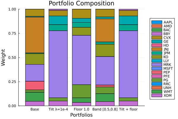
This page was generated using Literate.jl.