The source files can be found in examples/.
Windowed moment estimators
The estimators of the expected returns, covariance and higher moment pages used the whole return sample, with equal weight on each observation. That is the right default when the process that makes the returns does not change. In markets the process changes. Volatility comes in clusters and correlations rise in a crisis, and the risk of an asset today can differ a lot from its risk three years ago. A windowed estimator computes a moment from a chosen part of the history, or weights some observations more than others, instead of using the full sample with equal weights.
Each moment estimator has a windowed form: WindowedExpectedReturns, WindowedCovariance, WindowedVariance, WindowedCoskewness and WindowedCokurtosis. Each wraps a plain estimator of its moment, such as ce for the covariance or me for the mean, and adds two keywords.
windowis an integer or a vector of indices. An integer uses the lastwindowobservations. A vector uses the observations at those indices, which is a period you pick.wholds optional observation weights, such aseweights, which give older observations less weight without a hard cutoff.
Each call returns one moment, a mean vector or a covariance matrix, for the selected window. The estimator does not make a rolling time series. To move a window through time you write the loop yourself, as the last section shows.
Reach for a windowed estimator when you think that recent data tells you more than old data. Use a short trailing window or eweights for that. Use a vector window when you want a moment over one past episode, such as a crisis or a calm quarter. If you think that the full sample represents the future, the plain estimators of the earlier pages are the right default.
using PortfolioOptimisers, CSV, TimeSeries, DataFrames, Statistics, StatsBase, StatsPlots, PrettyTables, LinearAlgebra, Clarabelresfmt = (v, i, j) -> begin if j == 1 return v else return isa(v, Number) ? "$(round(v * 100, digits = 2)) %" : v endend;1. Data
The windows must differ for the comparison to show anything, so we take a longer slice than the other examples, about four years of daily S&P 500 returns instead of one. The timestamps in rd.ts let us select the days of a calendar episode later.
X = TimeArray(CSV.File(joinpath(@__DIR__, "..", "SP500.csv.gz")); timestamp = :Date)[(end - 1008):end]rd = prices_to_returns(X)ReturnsResult
nx ┼ 20-element Vector{String}
X ┼ 1008×20 Matrix{Float64}
nf ┼ nothing
F ┼ nothing
nb ┼ nothing
B ┼ nothing
ne ┼ nothing
E ┼ nothing
ts ┼ 1008-element Vector{Date}
iv ┼ nothing
ivpa ┼ nothing
pnl ┼ AssetPanel
│ pf ┼ Vector{AbstractPanelField}: AbstractPanelField[]
│ amsk ┼ 1008×20 AllTrueMask
│ emsk ┴ 1008×20 AllTrueMask
2. The length of a trailing window
The simplest control is an integer window, and the estimator then uses only the last window observations. We print the annualised volatility of every asset for four trailing windows and for the full sample.
annvol(ce) = sqrt.(diag(cov(ce, rd.X))) .* sqrt(252)windows = [60, 120, 252, 504]vol_table = DataFrame(:asset => rd.nx)vol_table[!, "full"] = annvol(PortfolioOptimisersCovariance())for w in windows vol_table[!, "win=$w"] = annvol(WindowedCovariance(; window = w))endpretty_table(vol_table; formatters = [resfmt], title = "Annualised volatility by trailing-window length") Annualised volatility by trailing-window length
┌────────┬─────────┬─────────┬─────────┬─────────┬─────────┐
│ asset │ full │ win=60 │ win=120 │ win=252 │ win=504 │
│ String │ Float64 │ Float64 │ Float64 │ Float64 │ Float64 │
├────────┼─────────┼─────────┼─────────┼─────────┼─────────┤
│ AAPL │ 34.53 % │ 40.44 % │ 36.04 % │ 35.51 % │ 30.8 % │
│ AMD │ 55.25 % │ 60.98 % │ 55.88 % │ 60.97 % │ 52.61 % │
│ BAC │ 37.69 % │ 32.82 % │ 31.68 % │ 32.39 % │ 29.23 % │
│ BBY │ 41.79 % │ 47.78 % │ 44.65 % │ 45.24 % │ 39.8 % │
│ CVX │ 37.91 % │ 28.43 % │ 32.32 % │ 32.86 % │ 28.97 % │
│ GE │ 44.54 % │ 31.84 % │ 32.04 % │ 34.79 % │ 33.67 % │
│ HD │ 30.03 % │ 31.31 % │ 30.02 % │ 31.25 % │ 26.31 % │
│ JNJ │ 20.61 % │ 15.17 % │ 15.9 % │ 17.39 % │ 16.01 % │
│ JPM │ 34.11 % │ 28.97 % │ 28.3 % │ 29.8 % │ 25.95 % │
│ KO │ 22.94 % │ 18.74 % │ 17.81 % │ 19.64 % │ 17.56 % │
│ LLY │ 31.56 % │ 23.58 % │ 26.98 % │ 27.22 % │ 29.5 % │
│ MRK │ 24.0 % │ 19.66 % │ 19.75 % │ 19.9 % │ 21.83 % │
│ MSFT │ 31.66 % │ 40.93 % │ 36.02 % │ 35.14 % │ 29.03 % │
│ PEP │ 23.04 % │ 19.3 % │ 18.12 % │ 19.42 % │ 17.24 % │
│ PFE │ 27.61 % │ 26.05 % │ 24.21 % │ 26.96 % │ 26.54 % │
│ PG │ 22.44 % │ 16.82 % │ 20.24 % │ 21.93 % │ 18.55 % │
│ RRC │ 75.02 % │ 59.63 % │ 58.11 % │ 62.82 % │ 63.79 % │
│ UNH │ 31.24 % │ 23.36 % │ 22.89 % │ 24.33 % │ 21.92 % │
│ WMT │ 23.4 % │ 23.02 % │ 26.0 % │ 26.68 % │ 22.23 % │
│ XOM │ 36.2 % │ 28.8 % │ 31.77 % │ 35.04 % │ 32.35 % │
└────────┴─────────┴─────────┴─────────┴─────────┴─────────┘On this slice the 60-day estimate is well above the 504-day and full-sample estimates for most assets, because the last months were more volatile than the four-year average. A short window follows a change of regime fast but carries more noise. A long window carries less noise but follows a change slowly.
3. Exponential observation weights
A hard window cutoff gives the observation just inside the window its full weight, and the one just outside no weight. Observation weights remove that step. eweights(1:T, λ) builds weights that fall geometrically with the age of an observation, so the newest one weighs the most. We pass them through the w field of the estimator to get a full-sample moment that weights recent data more.
eweights returns a plain StatsBase.Weights, which does not support Bessel's bias correction. The default covariance applies that correction and throws an error on these weights. Set corrected = false on the inner SimpleCovariance when you pass w. The other way is to pass frequency, analytic or probability weights, which support the correction.
T = size(rd.X, 1)ew = eweights(1:T, 2 / (T + 1); scale = true)uncorrected = PortfolioOptimisersCovariance(; ce = GeneralCovariance(; ce = SimpleCovariance(; corrected = false)))vol_w = DataFrame("asset" => rd.nx, "full (equal)" => annvol(PortfolioOptimisersCovariance()), "eweights" => annvol(WindowedCovariance(; ce = uncorrected, w = ew)), "win=252" => annvol(WindowedCovariance(; window = 252)))pretty_table(vol_w; formatters = [resfmt], title = "Annualised volatility with equal weights, exponential weights and a 252-day window")Annualised volatility with equal weights, exponential weights and a 252-day window
┌────────┬──────────────┬──────────┬─────────┐
│ asset │ full (equal) │ eweights │ win=252 │
│ String │ Float64 │ Float64 │ Float64 │
├────────┼──────────────┼──────────┼─────────┤
│ AAPL │ 34.53 % │ 34.22 % │ 35.51 % │
│ AMD │ 55.25 % │ 55.31 % │ 60.97 % │
│ BAC │ 37.69 % │ 35.19 % │ 32.39 % │
│ BBY │ 41.79 % │ 42.24 % │ 45.24 % │
│ CVX │ 37.91 % │ 35.55 % │ 32.86 % │
│ GE │ 44.54 % │ 40.18 % │ 34.79 % │
│ HD │ 30.03 % │ 29.52 % │ 31.25 % │
│ JNJ │ 20.61 % │ 18.95 % │ 17.39 % │
│ JPM │ 34.11 % │ 31.85 % │ 29.8 % │
│ KO │ 22.94 % │ 21.2 % │ 19.64 % │
│ LLY │ 31.56 % │ 30.72 % │ 27.22 % │
│ MRK │ 24.0 % │ 23.1 % │ 19.9 % │
│ MSFT │ 31.66 % │ 32.06 % │ 35.14 % │
│ PEP │ 23.04 % │ 21.15 % │ 19.42 % │
│ PFE │ 27.61 % │ 27.82 % │ 26.96 % │
│ PG │ 22.44 % │ 21.33 % │ 21.93 % │
│ RRC │ 75.02 % │ 70.05 % │ 62.82 % │
│ UNH │ 31.24 % │ 27.94 % │ 24.33 % │
│ WMT │ 23.4 % │ 23.9 % │ 26.68 % │
│ XOM │ 36.2 % │ 35.61 % │ 35.04 % │
└────────┴──────────────┴──────────┴─────────┘The weighted estimate keeps every observation. At the decay rate 2 / (T + 1) the oldest observation keeps about a seventh of the weight of the newest, so the weighted estimate stays close to the equal-weight one.
4. Conditioning on a named historical episode
An integer window always uses the most recent observations. A vector window uses any indices you give it, so we can estimate a moment over one episode. We compute the volatility of every asset over the COVID crash of February to April 2020 and over a calm quarter in mid-2021, with the same estimator.
covid = findall(d -> Date("2020-02-19") <= d <= Date("2020-04-30"), rd.ts)calm = findall(d -> Date("2021-04-01") <= d <= Date("2021-06-30"), rd.ts)regime_vol = DataFrame("asset" => rd.nx, "crash (Feb-Apr 2020)" => annvol(WindowedCovariance(; window = covid)), "calm (2021 Q2)" => annvol(WindowedCovariance(; window = calm)), "full" => annvol(PortfolioOptimisersCovariance()))pretty_table(regime_vol; formatters = [resfmt], title = "Annualised volatility over the 2020 crash, a calm 2021 quarter and the full sample")Annualised volatility over the 2020 crash, a calm 2021 quarter and the full sample
┌────────┬──────────────────────┬────────────────┬─────────┐
│ asset │ crash (Feb-Apr 2020) │ calm (2021 Q2) │ full │
│ String │ Float64 │ Float64 │ Float64 │
├────────┼──────────────────────┼────────────────┼─────────┤
│ AAPL │ 76.92 % │ 21.05 % │ 34.53 % │
│ AMD │ 92.16 % │ 35.3 % │ 55.25 % │
│ BAC │ 102.88 % │ 21.97 % │ 37.69 % │
│ BBY │ 91.66 % │ 25.93 % │ 41.79 % │
│ CVX │ 113.99 % │ 25.01 % │ 37.91 % │
│ GE │ 97.24 % │ 26.61 % │ 44.54 % │
│ HD │ 87.69 % │ 18.17 % │ 30.03 % │
│ JNJ │ 59.52 % │ 13.19 % │ 20.61 % │
│ JPM │ 97.69 % │ 19.09 % │ 34.11 % │
│ KO │ 62.92 % │ 10.57 % │ 22.94 % │
│ LLY │ 66.46 % │ 31.89 % │ 31.56 % │
│ MRK │ 57.89 % │ 18.59 % │ 24.0 % │
│ MSFT │ 80.26 % │ 19.23 % │ 31.66 % │
│ PEP │ 75.02 % │ 12.35 % │ 23.04 % │
│ PFE │ 57.46 % │ 16.3 % │ 27.61 % │
│ PG │ 65.51 % │ 14.3 % │ 22.44 % │
│ RRC │ 140.81 % │ 67.61 % │ 75.02 % │
│ UNH │ 91.66 % │ 17.21 % │ 31.24 % │
│ WMT │ 58.42 % │ 15.28 % │ 23.4 % │
│ XOM │ 82.8 % │ 27.63 % │ 36.2 % │
└────────┴──────────────────────┴────────────────┴─────────┘The crash window gives several times the volatility of the calm window, and the full-sample estimate averages that difference away. With a vector window you can compute the moments you would get if the coming months looked like one past episode.
5. Windowed estimators inside a prior
A windowed estimator goes into a prior as a plain one does. Set the me and ce fields of an EmpiricalPrior to windowed estimators and give the prior to an optimiser. The prior is then an estimator and not a computed result, so we pass the ReturnsResult to optimise. We solve a MinimumRisk portfolio for each window length and print its largest weight and the number of assets it holds.
slv = Solver(; name = :clarabel, solver = Clarabel.Optimizer, settings = Dict("verbose" => false), check_sol = (; allow_local = true, allow_almost = true))function windowed_minrisk(w) pe = EmpiricalPrior(; me = WindowedExpectedReturns(; window = w), ce = WindowedCovariance(; window = w)) return optimise(MeanRisk(; obj = MinimumRisk(), opt = JuMPOptimiser(; pe = pe, slv = slv)), rd)endfull_book = optimise(MeanRisk(; obj = MinimumRisk(), opt = JuMPOptimiser(; pe = EmpiricalPrior(), slv = slv)), rd)books = [windowed_minrisk(w) for w in windows]concentration = DataFrame("window" => ["full"; string.(windows)], "max weight" => [maximum(full_book.w); [maximum(b.w) for b in books]], "assets held" => [count(>(1e-4), full_book.w); [count(>(1e-4), b.w) for b in books]])concfmt = (v, i, j) -> j == 2 && isa(v, Number) ? "$(round(v * 100, digits = 2)) %" : vpretty_table(concentration; formatters = [concfmt], title = "Minimum-risk concentration by estimation window")Minimum-risk concentration by estimation window
┌────────┬────────────┬─────────────┐
│ window │ max weight │ assets held │
│ String │ Float64 │ Int64 │
├────────┼────────────┼─────────────┤
│ full │ 27.63 % │ 8 │
│ 60 │ 34.1 % │ 5 │
│ 120 │ 44.56 % │ 7 │
│ 252 │ 36.97 % │ 10 │
│ 504 │ 29.54 % │ 14 │
└────────┴────────────┴─────────────┘The short windows give portfolios that hold fewer assets than the long windows and the full sample. A short-window covariance carries more noise, and the optimiser puts its weight in the few assets that looked least risky over that short window. The order is not strict. The 120-day portfolio has the largest single weight of all, so the noise of a short window also makes the weights less predictable.
6. Moving a window through time
A trailing window computed at every date shows how a moment changes over time. We compute the 252-day trailing volatility of AAPL at each date from day 252 on, and plot the series. The full-sample estimate gives one number for the whole period.
roll = 252rolling_vol = [sqrt(cov(WindowedCovariance(; window = roll), rd.X[1:t, :])[1, 1]) * sqrt(252) for t in roll:T]rolling_dates = rd.ts[roll:T]plot(rolling_dates, rolling_vol; label = "AAPL trailing 252-day vol", xlabel = "date", ylabel = "annualised volatility", legend = :topright, lw = 2, title = "AAPL 252-day trailing volatility by date")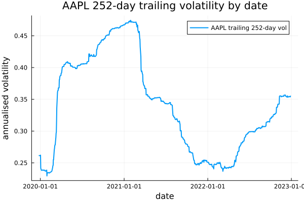
The volatility rises in early 2020, when the days of the COVID crash enter the trailing window. It falls 252 trading days later, when those days leave the window. A single windowed estimate is one point of this curve.
This page was generated using Literate.jl.