
The source files can be found in examples/.
Covariance estimation
The covariance matrix is the second moment that almost every optimiser depends on, and on a short window it is badly estimated: with
Denoising — separate signal from noise in the eigenspectrum.
DenoiseoffersFixedDenoise(collapse the sub-threshold bulk),ShrunkDenoise(shrink it) andSpectralDenoise(zero it) — the last does not always lower the condition number, as we will see.Sparsification — impose a relationship structure on the inverse.
LoGokeeps only the entries justified by the network topology, using a similarity measure such asMaximumDistanceSimilarityorExponentialSimilarity.
Both are configured through the MatrixProcessing pipeline on a PortfolioOptimisersCovariance, which is the ce field of a prior.
When to reach for this
Reach for covariance denoising/sparsification whenever your estimation window is short relative to the number of assets and you run anything that leans on the covariance — mean–variance, risk budgeting, clustering. A lower condition number means a more stable inverse and weights that move less when the data wobbles. Compare condition numbers before committing to a technique: SpectralDenoise in particular can make conditioning worse on some data.
using PortfolioOptimisers, PrettyTables, LinearAlgebra

mmtfmt = (v, i, j) -> begin
    if j == 1
        return v
    else
        return isa(v, Number) ? "$(round(v, digits=6))" : v
    end
end;
resfmt = (v, i, j) -> begin
    if j == 1
        return v
    else
        return isa(v, Number) ? "$(round(v*100, digits=3)) %" : v
    end
end;
1. ReturnsResult data
We use the same S&P 500 slice as the other examples.
using CSV, TimeSeries, DataFrames

X = TimeArray(CSV.File(joinpath(@__DIR__, "..", "SP500.csv.gz")); timestamp = :Date)[(end - 252):end]
rd = prices_to_returns(X)
ReturnsResult
nx ┼ 20-element Vector{String}
X ┼ 252×20 Matrix{Float64}
nf ┼ nothing
F ┼ nothing
nb ┼ nothing
B ┼ nothing
ts ┼ 252-element Vector{Date}
iv ┼ nothing
ivpa ┴ nothing2. Covariance estimators
We build one prior per covariance estimator, varying only the ce field (the expected returns are held at the plain sample mean). We compare the vanilla sample covariance against three denoisers and two LoGo sparsifications.
ces = ["Vanilla" => PortfolioOptimisersCovariance(),
       "FixedDenoise" => PortfolioOptimisersCovariance(;
                                                       mp = MatrixProcessing(;
                                                                             dn = Denoise(;
                                                                                          alg = FixedDenoise()))),
       "ShrunkDenoise" => PortfolioOptimisersCovariance(;
                                                        mp = MatrixProcessing(;
                                                                              dn = Denoise(;
                                                                                           alg = ShrunkDenoise(;
                                                                                                               alpha = 0.5)))),
       "SpectralDenoise" => PortfolioOptimisersCovariance(;
                                                          mp = MatrixProcessing(;
                                                                                dn = Denoise(;
                                                                                             alg = SpectralDenoise()))),
       "LoGo(MaxDist)" =>
           PortfolioOptimisersCovariance(; mp = MatrixProcessing(; alg = LoGo())),
       "LoGo(ExpDist)" => PortfolioOptimisersCovariance(;
                                                        mp = MatrixProcessing(;
                                                                              alg = LoGo(;
                                                                                         sim = ExponentialSimilarity())))]

prs = [k => prior(EmpiricalPrior(; ce = ce), rd) for (k, ce) in ces]
6-element Vector{Pair{String, LowOrderPrior{Matrix{Float64}, Vector{Float64}, Matrix{Float64}, Nothing, Nothing, Nothing, Nothing, Nothing, Nothing, Nothing, Nothing, Nothing}}}:
"Vanilla" => LowOrderPrior
X ┼ 252×20 Matrix{Float64}
mu ┼ 20-element Vector{Float64}
sigma ┼ 20×20 Matrix{Float64}
chol ┼ nothing
w ┼ nothing
ens ┼ nothing
kld ┼ nothing
ow ┼ nothing
rr ┼ nothing
f_mu ┼ nothing
f_sigma ┼ nothing
f_w ┴ nothing
"FixedDenoise" => LowOrderPrior
X ┼ 252×20 Matrix{Float64}
mu ┼ 20-element Vector{Float64}
sigma ┼ 20×20 Matrix{Float64}
chol ┼ nothing
w ┼ nothing
ens ┼ nothing
kld ┼ nothing
ow ┼ nothing
rr ┼ nothing
f_mu ┼ nothing
f_sigma ┼ nothing
f_w ┴ nothing
"ShrunkDenoise" => LowOrderPrior
X ┼ 252×20 Matrix{Float64}
mu ┼ 20-element Vector{Float64}
sigma ┼ 20×20 Matrix{Float64}
chol ┼ nothing
w ┼ nothing
ens ┼ nothing
kld ┼ nothing
ow ┼ nothing
rr ┼ nothing
f_mu ┼ nothing
f_sigma ┼ nothing
f_w ┴ nothing
"SpectralDenoise" => LowOrderPrior
X ┼ 252×20 Matrix{Float64}
mu ┼ 20-element Vector{Float64}
sigma ┼ 20×20 Matrix{Float64}
chol ┼ nothing
w ┼ nothing
ens ┼ nothing
kld ┼ nothing
ow ┼ nothing
rr ┼ nothing
f_mu ┼ nothing
f_sigma ┼ nothing
f_w ┴ nothing
"LoGo(MaxDist)" => LowOrderPrior
X ┼ 252×20 Matrix{Float64}
mu ┼ 20-element Vector{Float64}
sigma ┼ 20×20 Matrix{Float64}
chol ┼ nothing
w ┼ nothing
ens ┼ nothing
kld ┼ nothing
ow ┼ nothing
rr ┼ nothing
f_mu ┼ nothing
f_sigma ┼ nothing
f_w ┴ nothing
"LoGo(ExpDist)" => LowOrderPrior
X ┼ 252×20 Matrix{Float64}
mu ┼ 20-element Vector{Float64}
sigma ┼ 20×20 Matrix{Float64}
chol ┼ nothing
w ┼ nothing
ens ┼ nothing
kld ┼ nothing
ow ┼ nothing
rr ┼ nothing
f_mu ┼ nothing
f_sigma ┼ nothing
f_w ┴ nothingThe condition number is our headline diagnostic — lower is better-posed. FixedDenoise gives the biggest improvement here, while SpectralDenoise actually makes conditioning dramatically worse on this data, a reminder to always measure rather than assume.
pretty_table(DataFrame(; :estimator => [k for (k, _) in prs],
                       Symbol("cond(sigma)") => [cond(p.sigma) for (_, p) in prs]);
             formatters = [mmtfmt], title = "Covariance conditioning by estimator")
Covariance conditioning by estimator
┌─────────────────┬───────────────────────┐
│ estimator │ cond(sigma) │
│ String │ Float64 │
├─────────────────┼───────────────────────┤
│ Vanilla │ 177.278571 │
│ FixedDenoise │ 87.203326 │
│ ShrunkDenoise │ 135.392386 │
│ SpectralDenoise │ 4.5958939681259016e13 │
│ LoGo(MaxDist) │ 157.814013 │
│ LoGo(ExpDist) │ 159.846418 │
└─────────────────┴───────────────────────┘3. Visualising the eigenspectrum
plot_eigenspectrum shows the Marchenko–Pastur
Eigenspectrum: vanilla sample covariance.
using StatsPlots, GraphRecipesEigenspectrum: fixed-denoised covariance.
plot_eigenspectrum(prs[1].second, rd)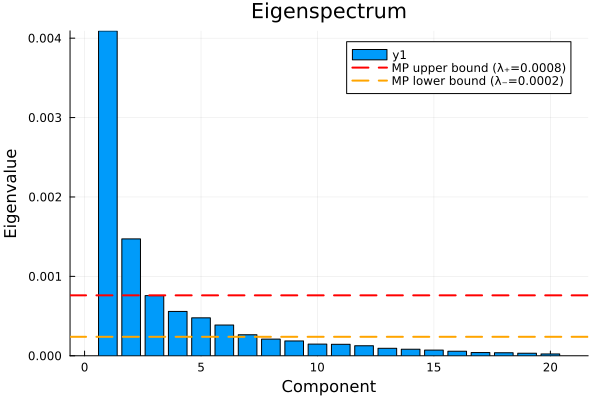
Eigenspectrum: LoGo(MaxDist) sparsified covariance.
plot_eigenspectrum(prs[2].second, rd)
plot_eigenspectrum(prs[5].second, rd)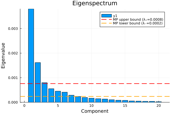
4. Why it matters: minimum-variance optimisation
Minimum-variance is the optimisation most exposed to covariance conditioning. We solve it with each prior and compare the weights — better-conditioned estimators produce more stable, less concentrated allocations.
using Clarabel

slv = Solver(; name = :clarabel1, solver = Clarabel.Optimizer,
             settings = Dict("verbose" => false),
             check_sol = (; allow_local = true, allow_almost = true))

ress = [k => optimise(MeanRisk(; r = Variance(), obj = MinimumRisk(),
                               opt = JuMPOptimiser(; pe = p, slv = slv))) for (k, p) in prs]

pretty_table(DataFrame(["Assets" => rd.nx; [k => r.w for (k, r) in ress]]);
             formatters = [resfmt],
             title = "Minimum-variance weights by covariance estimator")
Minimum-variance weights by covariance estimator
┌────────┬──────────┬──────────────┬───────────────┬─────────────────┬──────────
│ Assets │ Vanilla │ FixedDenoise │ ShrunkDenoise │ SpectralDenoise │ LoGo(Ma ⋯
│ String │ Float64 │ Float64 │ Float64 │ Float64 │ F ⋯
├────────┼──────────┼──────────────┼───────────────┼─────────────────┼──────────
│ AAPL │ 0.0 % │ 0.0 % │ 0.0 % │ 0.0 % │ ⋯
│ AMD │ 0.0 % │ 0.0 % │ 0.0 % │ 0.0 % │ ⋯
│ BAC │ 0.0 % │ 0.0 % │ 0.0 % │ 0.0 % │ ⋯
│ BBY │ 0.0 % │ 0.0 % │ 0.0 % │ 0.0 % │ ⋯
│ CVX │ 7.432 % │ 8.38 % │ 8.324 % │ 17.488 % │ 7 ⋯
│ GE │ 0.806 % │ 0.0 % │ 1.009 % │ 0.0 % │ ⋯
│ HD │ 0.0 % │ 0.0 % │ 0.0 % │ 0.0 % │ 5 ⋯
│ JNJ │ 36.974 % │ 35.168 % │ 38.354 % │ 76.031 % │ 32 ⋯
│ JPM │ 0.749 % │ 1.22 % │ 1.945 % │ 0.0 % │ 7 ⋯
│ KO │ 11.161 % │ 10.78 % │ 9.521 % │ 0.0 % │ 11 ⋯
│ LLY │ 0.0 % │ 0.0 % │ 0.0 % │ 0.0 % │ ⋯
│ MRK │ 17.467 % │ 15.754 % │ 16.628 % │ 0.0 % │ 19 ⋯
│ MSFT │ 0.0 % │ 0.0 % │ 0.0 % │ 0.0 % │ ⋯
│ PEP │ 8.978 % │ 12.167 % │ 8.038 % │ 0.0 % │ 1 ⋯
│ ⋮ │ ⋮ │ ⋮ │ ⋮ │ ⋮ │ ⋱
└────────┴──────────┴──────────────┴───────────────┴─────────────────┴──────────
2 columns and 6 rows omittedThe composition plot contrasts the minimum-variance portfolios across estimators.
plot_stacked_bar_composition([r for (_, r) in ress], rd;
                             xticks = (1:length(ress), [k for (k, _) in ress]))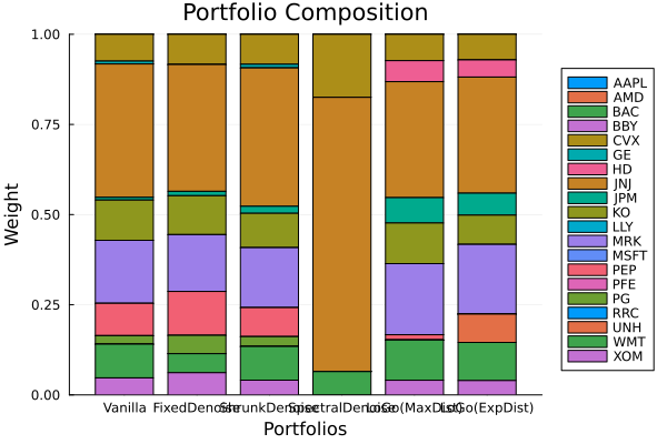
This page was generated using Literate.jl.