The source files can be found in examples/.
ℓ1 uncertainty sets: the quintile and 1/N portfolios
Two portfolios that practitioners use a lot have no theory behind them. The 1/N portfolio puts a weight of 1/N in each asset and uses no data. The quintile portfolio sorts the assets on a characteristic, such as momentum or low volatility, and holds the top 20 % with equal weights. Some versions also short the bottom 20 %. Both look naive, and both often do better than the portfolios that come from theory.
Zhou and Palomar [4] show that both are the exact solutions of a robust optimisation problem. The problem maximises the worst-case characteristic of the portfolio, when the true characteristic lies in an ℓ1 ball around your estimate. The radius ε of the ball is the only parameter, and it sets how many assets the portfolio holds.
| radius | portfolio | active assets |
|---|---|---|
ε → 0 | the best single asset | 1 |
ε moderate | the quintile portfolio | about 20 % of the assets |
ε large | the 1/N portfolio | all the assets, with equal weights |
You get the quintile portfolio when you believe your forecast in part, and the 1/N portfolio when you do not believe it at all.
Because the quintile portfolio is the solution of a robust problem, the library has no quintile optimiser. An ℓ1 ball is an uncertainty set, so the quintile portfolio is a MeanRisk problem with an ℓ1 ucs, and every constraint of the library applies to it. This page computes the sweep over ε behind the table above, the models of the paper, a ranking on a characteristic other than return, and the portfolios from theory that the paper compares with.
Reach for an ℓ1 set when you have a ranking that you trust in part. Do not set ε yourself, because its scale comes from the data, as section 3 shows. Give the number of assets you want to hold, and ActiveAssetsUncertaintyAlgorithm finds the radius. Reach for a box or ellipsoidal set instead when the size of the estimation error matters to you more than the order of the ranking.
using PortfolioOptimisers, PrettyTables, StatsPlots, Statistics, LinearAlgebra, HiGHS, Clarabelresfmt = (v, i, j) -> begin if j == 1 return v else return isa(v, AbstractFloat) ? "$(round(v*100, digits=2)) %" : v endend;1. Data and solver
We use the same S&P 500 slice as the other examples. The worst case over an ℓ1 ball is an infinity norm. One extra variable that bounds every entry makes an infinity norm linear. Every ℓ1 model of this page is a linear program, or a mixed-integer linear program in sections 7 and 8, and HiGHS solves both.
using CSV, TimeSeries, DataFramesX = TimeArray(CSV.File(joinpath(@__DIR__, "..", "SP500.csv.gz")); timestamp = :Date)[(end - 252):end]rd = prices_to_returns(X)pr = prior(EmpiricalPrior(), rd)slv = Solver(; name = :highs, solver = HiGHS.Optimizer, check_sol = (; allow_local = true, allow_almost = true), settings = Dict("log_to_console" => false))N = size(rd.X, 2)202. The model
The model has three parts.
ArithmeticReturnwith aucsmakes the return the worst case over the set, instead of the nominal return.MaximumReturnis the objective. The problem has no risk term.NoRiskis the risk measure that states this.
MeanRisk needs a risk measure. Without NoRisk it builds the default Variance, which the objective does not use. The variance still adds second-order cone constraints to the problem, and a conic solver is then necessary. NoRisk adds nothing to the model, so the problem stays a linear program.
function quintile(ucs; kwargs...) opt = JuMPOptimiser(; pe = pr, slv = slv, ret = ArithmeticReturn(; ucs = ucs), kwargs...) return optimise(MeanRisk(; opt = opt, r = NoRisk(), obj = MaximumReturn()))endlong_only(ucs) = quintile(ucs; bgt = 1.0, wb = WeightBounds(; lb = 0.0, ub = 1.0)).w;3. The scale of the radius comes from the data
ε has the units of a sum of differences of the characteristic, so its scale comes from the data and not from the model. On these daily returns the useful values are near 10⁻³, and on annualised returns they are about 250 times larger. No single value suits every data set. A value such as ε = 0.05 looks like a small 5 %, but here it is near the top of the range and gives almost the 1/N portfolio.
We print the radius that gives each of four portfolios, which hold one asset, 20 % of the assets, half of them and all of them. ladder(k) is the radius at which the k-th best asset joins the portfolio, from Lemma 2 of the paper, so a radius between ladder(k) and ladder(k + 1) gives k assets. The last asset has no ladder(N + 1), so every radius past ladder(N) gives 1/N. At exactly ladder(N) the last asset can stay at zero, so the table prints 1.25 ladder(N), the radius that section 12 solves at.
mu_sorted = sort(pr.mu; rev = true)ladder(k) = sum(mu_sorted[i] - mu_sorted[k] for i in 1:k)pretty_table(DataFrame(; portfolio = ["single best asset", "quintile (20%)", "half (50%)", "1/N (everything)"], radius = [ladder(2) / 2, (ladder(4) + ladder(5)) / 2, (ladder(10) + ladder(11)) / 2, ladder(N) * 1.25]); formatters = [(v, i, j) -> isa(v, Number) ? string(round(v; sigdigits = 3)) : v])┌───────────────────┬──────────┐
│ portfolio │ radius │
│ String │ Float64 │
├───────────────────┼──────────┤
│ single best asset │ 0.000346 │
│ quintile (20%) │ 0.00213 │
│ half (50%) │ 0.0107 │
│ 1/N (everything) │ 0.0739 │
└───────────────────┴──────────┘You do not need to find these radii by hand. ActiveAssetsUncertaintyAlgorithm inverts the closed forms of the paper. You give it the number of assets you want to hold, as a count or as a fraction, and it finds the radius. We build the set for 20 % of the assets.
active = 0.2 selects the radius that makes 20 % of the assets active on the problem with only the budget and the sign constraints. If you add weight bounds, a cardinality constraint or sector constraints, the number of active assets can differ. If you need a hard bound on the number of assets, use card.
ue = CharacteristicUncertaintySet(; pe = EmpiricalPrior(), alg = L1UncertaintySetAlgorithm(; method = ActiveAssetsUncertaintyAlgorithm(; active = 0.2)))mu_ucs(ue, rd)L1UncertaintySet
eps ┼ Float64: 0.0021257470647240177
sd ┼ nothing
mu ┴ 20-element Vector{Float64}
4. The sweep over ε
We compute the radius for each count of active assets from 1 to N, solve the long-only portfolio at each radius, and print six of the rows. As the radius grows, the portfolio moves from a single asset to 1/N. The quintile portfolio is the exact optimum at a radius between the two.
targets = 1:Nsweep = map(targets) do q alg = L1UncertaintySetAlgorithm(; method = ActiveAssetsUncertaintyAlgorithm(; active = q)) eps = mu_ucs(CharacteristicUncertaintySet(; alg = alg), rd).eps w = long_only(L1UncertaintySet(; eps = eps)) return (; q = q, eps = eps, active = count(>(1e-6), w), max_weight = maximum(w), hhi = sum(abs2, w))endsweep_df = DataFrame(sweep)pretty_table(sweep_df[[1, 2, 4, 8, 12, 20], :]; formatters = [(v, i, j) -> if isa(v, AbstractFloat) string(round(v; sigdigits = 3)) else v end])┌───────┬──────────┬────────┬────────────┬─────────┐
│ q │ eps │ active │ max_weight │ hhi │
│ Int64 │ Float64 │ Int64 │ Float64 │ Float64 │
├───────┼──────────┼────────┼────────────┼─────────┤
│ 1 │ 0.000346 │ 1 │ 1.0 │ 1.0 │
│ 2 │ 0.000813 │ 2 │ 0.5 │ 0.5 │
│ 4 │ 0.00213 │ 4 │ 0.25 │ 0.25 │
│ 8 │ 0.00795 │ 8 │ 0.125 │ 0.125 │
│ 12 │ 0.014 │ 12 │ 0.0833 │ 0.0833 │
│ 20 │ 0.0744 │ 20 │ 0.05 │ 0.05 │
└───────┴──────────┴────────┴────────────┴─────────┘Read the active column against q, and max_weight against 1/q. On each printed row they are equal, so the portfolio holds equal weights over its active assets, as the quintile portfolio does. We plot the number of active assets against the radius.
plot(sweep_df.eps, sweep_df.active; label = "active assets", xlabel = "uncertainty radius ε", ylabel = "number of active assets", legend = :bottomright, marker = :circle, markersize = 2)hline!([N]; label = "1/N portfolio", linestyle = :dash)hline!([round(Int, 0.2 * N)]; label = "quintile (20%)", linestyle = :dash)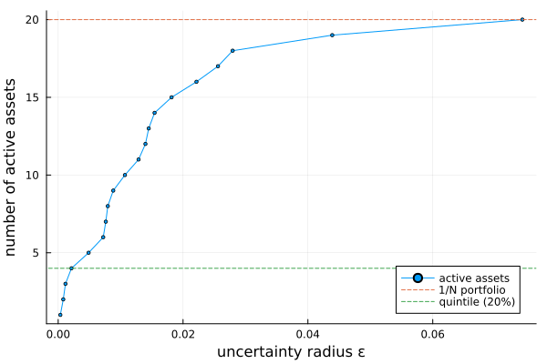
5. Equal weights or inverse volatility
The ball above assumes the same error in the estimate of each asset's characteristic. But the mean return of a volatile asset is harder to estimate than that of a calm one. The set A₁ of the paper scales the ball by the volatility of each asset. The active assets then take weights in inverse proportion to their volatility, instead of equal weights. Only the shape of the ball changes, and the objective and the constraints stay the same.
With the estimator, scaled = true on L1UncertaintySetAlgorithm gives this set. Here we build the set directly and pass the volatilities as sd. We solve both portfolios at the quintile radius, and print their weights next to the inverse-volatility weights that Lemma 9 of the paper predicts. gs(k) is the ladder of the scaled set: it divides each difference mu_sorted[i] - mu_sorted[k] of ladder(k) by the volatility of asset i.
sd_hat = sqrt.(diag(pr.sigma))sd_by_mu = sd_hat[sortperm(pr.mu; rev = true)]gs(k) = sum((mu_sorted[i] - mu_sorted[k]) / sd_by_mu[i] for i in 1:k)w_equal = long_only(L1UncertaintySet(; eps = (ladder(4) + ladder(5)) / 2))w_invvol = long_only(L1UncertaintySet(; eps = (gs(4) + gs(5)) / 2, sd = sd_hat))act = findall(>(1e-6), w_invvol)pretty_table(DataFrame(; asset = rd.nx[act], volatility = sd_hat[act], equal_weighted = w_equal[act], inverse_vol = w_invvol[act], predicted = (1 ./ sd_hat[act]) ./ sum(1 ./ sd_hat[act])); formatters = [resfmt])┌────────┬────────────┬────────────────┬─────────────┬───────────┐
│ asset │ volatility │ equal_weighted │ inverse_vol │ predicted │
│ String │ Float64 │ Float64 │ Float64 │ Float64 │
├────────┼────────────┼────────────────┼─────────────┼───────────┤
│ CVX │ 2.07 % │ 25.0 % │ 24.32 % │ 24.32 % │
│ MRK │ 1.25 % │ 25.0 % │ 40.15 % │ 40.15 % │
│ RRC │ 3.96 % │ 25.0 % │ 12.72 % │ 12.72 % │
│ XOM │ 2.21 % │ 25.0 % │ 22.81 % │ 22.81 % │
└────────┴────────────┴────────────────┴─────────────┴───────────┘Compare the inverse_vol column with predicted. Lemma 9 of the paper states that the two are equal, and the table prints the same digits in both. At a larger radius every asset is active, and the weights are the inverse-volatility weights of all the assets, the counterpart of 1/N. The cell prints true if the weights are within 1e-6 of those.
w_iv_all = long_only(L1UncertaintySet(; eps = gs(N) * 1.5, sd = sd_hat))isapprox(w_iv_all, (1 ./ sd_hat) ./ sum(1 ./ sd_hat); atol = 1e-6)true6. The dollar-neutral long-short quintile
The long-short quintile portfolio is long the top assets and short the bottom ones. The paper needs the antisymmetric pairing of its Lemma 5 to solve it. Here it takes two budgets. bgt = 0 makes the portfolio dollar-neutral, and sbgt = 0.5 puts half the gross exposure on each side. In the solution, the i-th best asset is long and the i-th worst is short, at equal and opposite weights, and no constraint of the model imposes that pairing.
function f(m) return sum(mu_sorted[i] - mu_sorted[m] for i in 1:m) + sum(mu_sorted[N - m + 1] - mu_sorted[N - j + 1] for j in 1:m)endw_ls = quintile(L1UncertaintySet(; eps = (f(4) + f(5)) / 2); bgt = 0.0, sbgt = 0.5, wb = WeightBounds(; lb = -1.0, ub = 1.0)).wnz = findall(>(1e-6), abs.(w_ls))pretty_table(DataFrame(; asset = rd.nx[nz], weight = w_ls[nz], side = ifelse.(w_ls[nz] .> 0, "long", "short")); formatters = [resfmt])┌────────┬─────────┬────────┐
│ asset │ weight │ side │
│ String │ Float64 │ String │
├────────┼─────────┼────────┤
│ AAPL │ -12.5 % │ short │
│ AMD │ -12.5 % │ short │
│ BAC │ -12.5 % │ short │
│ CVX │ 12.5 % │ long │
│ MRK │ 12.5 % │ long │
│ MSFT │ -12.5 % │ short │
│ RRC │ 12.5 % │ long │
│ XOM │ 12.5 % │ long │
└────────┴─────────┴────────┘The table shows four long and four short positions. Corollary 7 of the paper gives each weight as ±1/(2m), the net exposure as zero and the gross exposure as one.
(net = sum(w_ls), gross = sum(abs, w_ls))(net = 0.0, gross = 1.0)7. The short and gross budgets are upper bounds
This section applies to every model built on a JuMPOptimiser. A number for bgt fixes the net exposure sum(w). The long and short variables are upper bounds on the positive and negative parts of w, so sbgt = 0.3 means at most 30 % short. You do not usually see the difference, because the objective pushes the exposure to the budget.
You see it at a very large radius. Past the radius at which every asset is active, the worst-case return of the 50/50 portfolio is negative. The paper still holds that portfolio, because its constraint ‖w‖₁ = 1 requires full investment. The problem here only bounds the exposure, so its optimum is to hold nothing. A portfolio of zeros is of no use, and the library returns an optimisation failure instead. The cell prints true if the return code is an OptimisationFailure.
eps_extreme = f(N ÷ 2) * 1.5relaxed = quintile(L1UncertaintySet(; eps = eps_extreme); bgt = 0.0, sbgt = 0.5, wb = WeightBounds(; lb = -1.0, ub = 1.0))isa(relaxed.jr.retcode, PortfolioOptimisers.OptimisationFailure)trueWith xbgt = true the long and the short parts of w equal their budgets, as in the paper. The portfolio stays fully invested and takes the worst-case loss.
exact = quintile(L1UncertaintySet(; eps = eps_extreme); bgt = 0.0, sbgt = 0.5, xbgt = true, wb = WeightBounds(; lb = -1.0, ub = 1.0))(retcode = typeof(exact.jr.retcode).name.name, gross = sum(abs, exact.w), active = count(>(1e-6), abs.(exact.w)))(retcode = :OptimisationSuccess, gross = 1.0000000000000002, active = 20)It adds a binary variable per asset for the sign of the weight, and the solver must search over the values of those variables. On twenty assets the solve takes seconds, and on a large universe it can take too long to be of use. card, lt, st and fixed fees build the same binary variables, so with any of them xbgt adds no new ones. Leave it off unless your problem requires full investment.
8. A market-neutral portfolio with a fixed gross exposure
A market-neutral portfolio needs βᵀw = 0 and a fixed gross exposure, and it leaves the net exposure free. bgt and sbgt constrain the net and the gross exposure together, so they cannot fix the gross exposure at one and leave the net free. gbgt constrains the gross exposure alone, so we use it here. Without it, only the weight bounds of -1 and 1 limit the gross exposure. gbgt bounds the gross exposure unless xbgt = true, so we set both.
The paper notes that the active assets no longer follow the order of the ranking here, so no closed form gives the weights. The solver still solves the problem, which xbgt = true makes a mixed-integer linear program. The paper assumes a positive market beta for each asset, so we take the correlation of each asset with the average return of all the assets, and add 0.5 to its absolute value.
beta = vec(cor(rd.X, mean(rd.X; dims = 2)))beta = abs.(beta) .+ 0.5lc_mn = LinearConstraint(; eq = PartialLinearConstraint(reshape(beta, 1, N), [0.0]))w_mn = quintile(L1UncertaintySet(; eps = 0.002); bgt = nothing, gbgt = 1.0, xbgt = true, lcse = lc_mn, wb = WeightBounds(; lb = -1.0, ub = 1.0)).w(gross = sum(abs, w_mn), net = sum(w_mn), market_exposure = dot(beta, w_mn))(gross = 1.0000000000000002, net = 0.09472668024976366, market_exposure = 0.0)The gross exposure is one and the market exposure is zero. The net exposure is whatever the optimum gives.
9. A characteristic other than a return
The paper states that the construction works for any characteristic of an asset, and its Table III ranks the assets on their estimated volatility.
Put the characteristic in the return term. The mu field of ArithmeticReturn takes the vector, or the estimator that computes it, as here. The optimiser computes the vector from its own prior when it builds the model. If you give the estimator instead of a vector, the ranking is computed again for each cross-validation fold and for each subset of a meta-optimiser. We rank on volatility and print the volatility and the weight of each active asset.
w_vol = optimise(MeanRisk(; r = NoRisk(), obj = MaximumReturn(), opt = JuMPOptimiser(; pe = pr, slv = slv, bgt = 1.0, wb = WeightBounds(; lb = 0.0, ub = 1.0), ret = ArithmeticReturn(; mu = StandardDeviationExpectedReturns(), ucs = L1UncertaintySet(; eps = 0.05))))).wsd_assets = sqrt.(diag(pr.sigma))act_vol = findall(>(1e-6), w_vol)pretty_table(DataFrame(; asset = rd.nx[act_vol], volatility = sd_assets[act_vol], weight = w_vol[act_vol]); formatters = [resfmt])┌────────┬────────────┬─────────┐
│ asset │ volatility │ weight │
│ String │ Float64 │ Float64 │
├────────┼────────────┼─────────┤
│ AAPL │ 2.24 % │ 14.29 % │
│ AMD │ 3.84 % │ 14.29 % │
│ BBY │ 2.85 % │ 14.29 % │
│ GE │ 2.19 % │ 14.29 % │
│ MSFT │ 2.21 % │ 14.29 % │
│ RRC │ 3.96 % │ 14.29 % │
│ XOM │ 2.21 % │ 14.29 % │
└────────┴────────────┴─────────┘You can also rank on volatility if you build the prior with StandardDeviationExpectedReturns and give the return term no mu. On this page the two ways give the same weights, because with NoRisk nothing else uses μ. When something else uses it, they differ. Every moment risk measure centres on the prior's μ, and so do the value-at-risk measures and the normalisation of MaximumRatio. With a mean-centred risk measure in place of NoRisk, the measure then computes deviations about a vector of volatilities. The same problem gives a different portfolio, and no warning tells you. The prior's μ is the vector of expected returns. A ranking is not an expected return, so put it in the return term.
The objective maximises the characteristic. With a ranking on volatility, the most volatile assets come first. The low-volatility factor of the paper needs the opposite order. If a smaller value of a characteristic is better, negate it. Here we pass the mu field a plain vector, the negated volatilities.
lowvol = ArithmeticReturn(; mu = -sd_assets, ucs = L1UncertaintySet(; eps = 0.05))w_lowvol = optimise(MeanRisk(; r = NoRisk(), obj = MaximumReturn(), opt = JuMPOptimiser(; pe = pr, slv = slv, bgt = 1.0, wb = WeightBounds(; lb = 0.0, ub = 1.0), ret = lowvol))).wact_lv = findall(>(1e-6), w_lowvol)pretty_table(DataFrame(; asset = rd.nx[act_lv], volatility = sd_assets[act_lv], weight = w_lowvol[act_lv]); formatters = [resfmt])┌────────┬────────────┬─────────┐
│ asset │ volatility │ weight │
│ String │ Float64 │ Float64 │
├────────┼────────────┼─────────┤
│ HD │ 1.97 % │ 9.09 % │
│ JNJ │ 1.1 % │ 9.09 % │
│ JPM │ 1.88 % │ 9.09 % │
│ KO │ 1.24 % │ 9.09 % │
│ LLY │ 1.71 % │ 9.09 % │
│ MRK │ 1.25 % │ 9.09 % │
│ PEP │ 1.22 % │ 9.09 % │
│ PFE │ 1.7 % │ 9.09 % │
│ PG │ 1.38 % │ 9.09 % │
│ UNH │ 1.53 % │ 9.09 % │
│ WMT │ 1.68 % │ 9.09 % │
└────────┴────────────┴─────────┘The portfolio holds the least volatile assets with equal weights, which is the low-volatility factor. We print the range of volatility of each selection and of all the assets. The two selections share no asset, and the only change between the two models is the sign of the characteristic.
(ranked_on_high_vol = round.(extrema(sd_assets[act_vol]); sigdigits = 3), ranked_on_low_vol = round.(extrema(sd_assets[act_lv]); sigdigits = 3), universe = round.(extrema(sd_assets); sigdigits = 3))(ranked_on_high_vol = (0.0219, 0.0396), ranked_on_low_vol = (0.011, 0.0197), universe = (0.011, 0.0396))10. Several terms at once, and what a floor costs
One model can have a term for a ranking and a term for the expected return. ret takes a vector of return terms, as r takes a vector of risk measures. The return of the model is the weighted sum Σᵢ scaleᵢ · retᵢ of the terms. The sca field of JuMPOptimiser lets you choose how several risk measures combine, and the return side has no such choice.
A term can also stay out of that sum. Each term has a JuMPReturnsSettings, and rte = false keeps the term out of the objective while its lb still constrains the portfolio. Such a term changes the feasible set and adds nothing to the objective.
We use it to find what a floor on the expected return costs the low-volatility portfolio above. The floor term has no mu of its own, so it uses the prior's μ, the vector of expected returns. A volatility ranking in the prior would replace that value. We solve at four floors and print the number of assets, the expected return and the average volatility of each portfolio.
floor_term(lb) = ArithmeticReturn(; settings = JuMPReturnsSettings(; rte = false, lb = lb))function lowvol_with_floor(lb) return optimise(MeanRisk(; r = NoRisk(), obj = MaximumReturn(), opt = JuMPOptimiser(; pe = pr, slv = slv, bgt = 1.0, wb = WeightBounds(; lb = 0.0, ub = 1.0), ret = [lowvol, floor_term(lb)]))).wendfloors = [0.0, 0.0005, 0.001, 0.0015]ws = [iszero(lb) ? w_lowvol : lowvol_with_floor(lb) for lb in floors]pretty_table(DataFrame(; floor = ["none", "0.05 %", "0.10 %", "0.15 %"], names = [count(>(1e-6), w) for w in ws], expected_return = [dot(pr.mu, w) for w in ws], avg_volatility = [dot(sd_assets, w) for w in ws]); formatters = [resfmt])┌────────┬───────┬─────────────────┬────────────────┐
│ floor │ names │ expected_return │ avg_volatility │
│ String │ Int64 │ Float64 │ Float64 │
├────────┼───────┼─────────────────┼────────────────┤
│ none │ 11 │ 0.03 % │ 1.51 % │
│ 0.05 % │ 11 │ 0.05 % │ 1.51 % │
│ 0.10 % │ 10 │ 0.1 % │ 1.52 % │
│ 0.15 % │ 6 │ 0.15 % │ 1.65 % │
└────────┴───────┴─────────────────┴────────────────┘At each of the three floors, the expected_return column equals the floor, so the floor constraint is active. As the floor rises, the portfolio holds fewer assets and their average volatility rises. That is the cost of the floor in the units of the first term, and neither term alone can show it.
When a model has several terms, two rules apply.
scaleis a weight and does not normalise. The model sums the terms as written, so two terms are averaged only if you halve both. Fees follow the same sum. A term charges fees only if itsfeeflag istrue. Two such terms atscale = 1subtract the fees twice. Setfee, andmic, the flag for the market impact cost, tofalseon any term that is not in units of return.rte = falseserves two cases. A term that is not in units of return does not belong in a sum of returns. A term in units of return, such as the floor above, can also be wanted as a bound alone. The flag says only that the term stays out of the objective, and itslbconstrains the portfolio in both cases.
11. The quintile portfolio with other constraints
Section 2 built the quintile portfolio as a MeanRisk model, and a weight bound constrains it as it constrains any other model. We cap each weight at 15 %, and print the number of active assets and the largest weight with and without the cap.
eps_q = (ladder(4) + ladder(5)) / 2w_free = long_only(L1UncertaintySet(; eps = eps_q))w_capped = quintile(L1UncertaintySet(; eps = eps_q); bgt = 1.0, wb = WeightBounds(; lb = 0.0, ub = 0.15)).wpretty_table(DataFrame(; portfolio = ["unconstrained", "capped at 15%"], active = [count(>(1e-6), w_free), count(>(1e-6), w_capped)], largest = [maximum(w_free), maximum(w_capped)]); formatters = [resfmt])┌───────────────┬────────┬─────────┐
│ portfolio │ active │ largest │
│ String │ Int64 │ Float64 │
├───────────────┼────────┼─────────┤
│ unconstrained │ 4 │ 25.0 % │
│ capped at 15% │ 7 │ 15.0 % │
└───────────────┴────────┴─────────┘With the cap, the portfolio no longer holds the four assets that the radius was chosen for. This is the case of the warning in section 3. The radius gives four assets on the problem without the cap, and the cap changes the problem.
12. The benchmarks
The paper compares these portfolios with four portfolios from theory, and each is a MeanRisk model. GMVP is the global minimum variance portfolio, MVP the mean-variance portfolio, MSRP the maximum Sharpe ratio portfolio and GMRP the global maximum return portfolio. GMRP maximises return with no risk term. It uses NoRisk as section 2 does, and it is the limit of the ℓ1 portfolios as ε → 0.
Three of the four have a variance term, which needs a conic solver, so we solve all four with Clarabel. The ℓ1 models of this page have no variance term, and HiGHS solves them.
cslv = Solver(; name = :clarabel, solver = Clarabel.Optimizer, check_sol = (; allow_local = true, allow_almost = true), settings = Dict("verbose" => false))function lo_opt(; kwargs...) return JuMPOptimiser(; pe = pr, slv = cslv, bgt = 1.0, wb = WeightBounds(; lb = 0.0, ub = 1.0), kwargs...)endbenchmarks = Dict("GMVP (min variance)" => MeanRisk(; opt = lo_opt(), r = Variance(), obj = MinimumRisk()), "MVP (mean-variance)" => MeanRisk(; opt = lo_opt(), r = Variance(), obj = MaximumUtility(; l = 25.0)), "GMRP (max return)" => MeanRisk(; opt = lo_opt(), r = NoRisk(), obj = MaximumReturn()), "MSRP (max Sharpe)" => MeanRisk(; opt = lo_opt(), r = Variance(), obj = MaximumRatio()));We solve the four and put them in one table with the ℓ1 portfolios of this page. As in the paper, the comparison is in sample, on the same estimates that built every portfolio. It shows what each objective does, and it says nothing about performance out of sample.
#! At exactly `ladder(N)` the last asset can stay at zero, so take a radius past it for 1/N.w_1n = long_only(L1UncertaintySet(; eps = ladder(N) * 1.25))rows = [(; portfolio = name, w = optimise(mre).w) for (name, mre) in sort(collect(benchmarks); by = first)]append!(rows, [(; portfolio = "1/N (ε large)", w = w_1n), (; portfolio = "quintile (ε mid)", w = w_free), (; portfolio = "inverse vol (ε large, scaled)", w = w_iv_all)])bench_df = DataFrame(; portfolio = [r.portfolio for r in rows], ret = [dot(pr.mu, r.w) for r in rows], vol = [sqrt(dot(r.w, pr.sigma, r.w)) for r in rows], sharpe = [dot(pr.mu, r.w) / sqrt(dot(r.w, pr.sigma, r.w)) for r in rows], active = [count(>(1e-6), r.w) for r in rows], largest = [maximum(r.w) for r in rows])pretty_table(bench_df; formatters = [(v, i, j) -> if j == 4 string(round(v; sigdigits = 3)) elseif isa(v, AbstractFloat) "$(round(v*100, digits=3)) %" else v end])┌───────────────────────────────┬─────────┬─────────┬─────────┬────────┬──────────┐
│ portfolio │ ret │ vol │ sharpe │ active │ largest │
│ String │ Float64 │ Float64 │ Float64 │ Int64 │ Float64 │
├───────────────────────────────┼─────────┼─────────┼─────────┼────────┼──────────┤
│ GMRP (max return) │ 0.264 % │ 2.207 % │ 0.119 │ 1 │ 100.0 % │
│ GMVP (min variance) │ 0.077 % │ 0.934 % │ 0.0826 │ 11 │ 36.974 % │
│ MSRP (max Sharpe) │ 0.199 % │ 1.208 % │ 0.164 │ 10 │ 67.266 % │
│ MVP (mean-variance) │ 0.133 % │ 0.989 % │ 0.134 │ 7 │ 42.871 % │
│ 1/N (ε large) │ 0.015 % │ 1.283 % │ 0.0115 │ 20 │ 5.0 % │
│ quintile (ε mid) │ 0.202 % │ 1.884 % │ 0.107 │ 4 │ 25.0 % │
│ inverse vol (ε large, scaled) │ 0.025 % │ 1.143 % │ 0.0215 │ 20 │ 8.175 % │
└───────────────────────────────┴─────────┴─────────┴─────────┴────────┴──────────┘Three benchmarks have the best value in the column of their own objective. GMVP has the lowest volatility, GMRP the highest return and MSRP the highest Sharpe ratio. MVP trades return against variance, and no column of the table is its objective. GMRP holds a single asset, which is the portfolio at ε → 0 in the sweep of section 4.
No ℓ1 portfolio has the best value in any of these three columns. 1/N and the inverse-volatility portfolio have the lowest returns and Sharpe ratios of the table. The three benchmarks optimise their own column on the same estimates that the table uses, so in sample no other portfolio can beat them there. An ℓ1 portfolio uses μ only in part and scores lower on the columns that μ computes.
The last two columns, active and largest, show how concentrated each portfolio is. GMRP and MSRP put most of their weight in few assets, and both act on 252 days of estimates as if the estimates were exact. The quintile portfolio and 1/N spread equal weights over four assets and over all of them. The in-sample columns do not measure the risk of a concentrated portfolio. Only a test out of sample can show whether the spread pays, and this page does not run one. The cross validation examples show how to run such a test.
13. What to take away
- The quintile and 1/N portfolios are the exact solutions of a robust optimisation problem over an ℓ1 ball. The radius
εsets how many assets the portfolio holds. - The library has no quintile optimiser. The quintile portfolio is
MeanRisk(; r = NoRisk(), obj = MaximumReturn())with an ℓ1ucs, so every constraint of the library applies to it. - The scale of
εcomes from the data. Give the number of assets toActiveAssetsUncertaintyAlgorithminstead, and expect other constraints to change that number. - A ball scaled by the volatility of each asset gives inverse-volatility weights where the plain ball gives equal weights, and the objective and the constraints stay the same.
- A number for
bgtfixes the net exposure.sbgtandgbgtbound the short and the gross exposure and do not fix them.xbgt = truefixes them and makes the problem mixed-integer. - The
mufield ofArithmeticReturnranks on any characteristic, as a vector or as the estimator that computes it. Put the characteristic in the return term and never in the prior, whoseμevery mean-centred risk measure centres on. The objective maximises, so negate a characteristic when a smaller value is better. rettakes several terms and sums them with their weights. A term withrte = falsestays out of the objective and keeps itslb, and section 10 uses one to show what a floor on the expected return costs.
This page was generated using Literate.jl.