The source files can be found in user_guide/.

Data and priors

The first pipeline stage turns raw prices into a prior — the expected-returns vector and covariance matrix every optimiser consumes. Two calls cover the common path: prices_to_returns and prior. This page is the quick tour; for the full menu of moment estimators and view-based priors, see the moments & priors examples.

using PortfolioOptimisers, CSV, TimeSeries, DataFrames, PrettyTables, LinearAlgebra,
      StatsPlots, GraphRecipes

resfmt = (v, i, j) -> begin
    return if j == 1
        v
    else
        isa(v, AbstractFloat) ? "$(round(v*100, digits=3)) %" : v
    end
end;

1. Prices to returns

Price data usually arrives from an API and must be converted to returns. prices_to_returns handles asset, factor, and benchmark prices (plus implied volatilities and volatility premiums), validates that the series are consistent, and can impute missing prices (Impute.jl) and collapse to lower frequencies (TimeSeries.jl). Given a single TimeArray of prices it returns a ReturnsResult holding the asset names nx and the return matrix X.

Real price tables are rarely clean — newly listed or delisted names leave leading/trailing gaps, halts and stale quotes leave flat stretches, and exchanges keep different holiday calendars. The missing_col_percent / missing_row_percent filters and impute_method handle all of it in this one call, before differencing prices into returns; the Data preprocessing and imputation example is the deep dive.

X = TimeArray(CSV.File(joinpath(@__DIR__, "../examples/SP500.csv.gz")); timestamp = :Date)[(end - 252):end]
rd = prices_to_returns(X)

ReturnsResult
    nx ┼ 20-element Vector{String}
     X ┼ 252×20 Matrix{Float64}
    nf ┼ nothing
     F ┼ nothing
    nb ┼ nothing
     B ┼ nothing
    ts ┼ 252-element Vector{Date}
    iv ┼ nothing
  ivpa ┴ nothing

When you also pass factor and benchmark price series, prices_to_returns aligns them on matching timestamps and carries the factor returns F and benchmark iv through on the same ReturnsResult — everything downstream then has the data it needs.

2. Returns to a prior

prior applies a prior estimator to a ReturnsResult and returns the moments. The blessed default is EmpiricalPrior — the sample mean and covariance.

pr = prior(EmpiricalPrior(), rd)

pretty_table(DataFrame("Asset" => rd.nx, "Expected return" => pr.mu,
                       "Volatility" => sqrt.(diag(pr.sigma))); formatters = [resfmt],
             title = "Empirical prior: per-asset mean and volatility")

Empirical prior: per-asset mean and volatility
┌────────┬─────────────────┬────────────┐
│  Asset │ Expected return │ Volatility │
│ String │         Float64 │    Float64 │
├────────┼─────────────────┼────────────┤
│   AAPL │        -0.113 % │    2.237 % │
│    AMD │        -0.281 % │     3.84 % │
│    BAC │        -0.093 % │     2.04 % │
│    BBY │        -0.028 % │     2.85 % │
│    CVX │         0.195 % │     2.07 % │
│     GE │        -0.034 % │    2.192 % │
│     HD │        -0.071 % │    1.968 % │
│    JNJ │         0.031 % │    1.096 % │
│    JPM │        -0.042 % │    1.877 % │
│     KO │          0.05 % │    1.237 % │
│    LLY │         0.131 % │    1.714 % │
│    MRK │         0.167 % │    1.254 % │
│   MSFT │        -0.121 % │    2.214 % │
│    PEP │         0.039 % │    1.223 % │
│      ⋮ │               ⋮ │          ⋮ │
└────────┴─────────────────┴────────────┘
                           6 rows omitted

3. Swapping the prior

EmpiricalPrior is only the starting point. Every prior estimator has the same prior(pe, rd) interface, so swapping one in is a one-line change. The common alternatives:

• FactorPrior — moments from a factor model (deep dive: Factor Priors).

• BlackLittermanPrior — blend market-equilibrium moments with your views (deep dive: Black–Litterman). The family extends to BayesianBlackLittermanPrior, FactorBlackLittermanPrior (views on factor premia) and AugmentedBlackLittermanPrior (asset and factor views together) — see Advanced Black–Litterman.

• EntropyPoolingPrior / OpinionPoolingPrior — reweight the empirical scenarios to satisfy views on any moment (deep dives: Entropy Pooling, Opinion Pooling).

The covariance estimator inside a prior is itself swappable (shrinkage, denoising, Gerber, …); see Covariance Estimation. Any moment estimator can also be windowed — restricted to a trailing window or recency-weighted — when the recent regime is more informative than the full sample (deep dive: Windowed Estimators; regime-adjusted estimators are a related sibling).

4. A first look at the data

plot_prior summarises a prior in one figure — expected returns, per-asset volatility, and the correlation matrix — a quick sanity check before optimising.

plot_prior(pr, rd)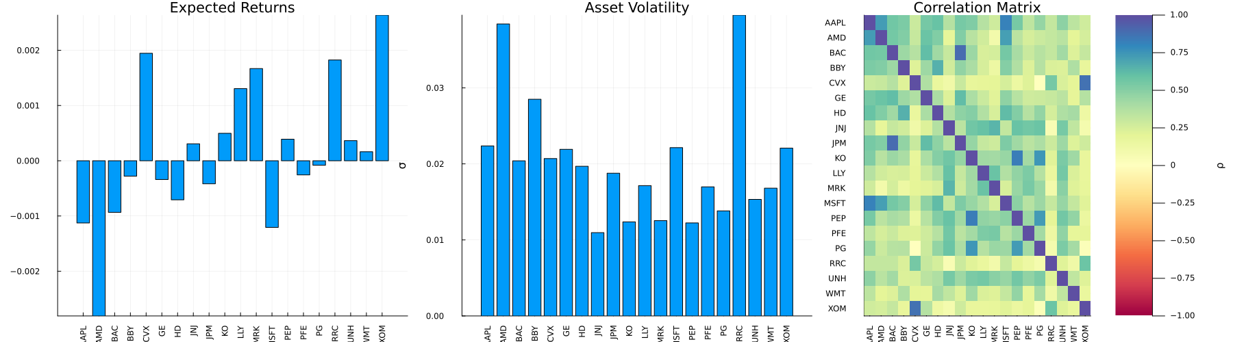

---

This page was generated using Literate.jl.