The source files can be found in examples/.

Profile: retail, daily

The earlier examples each isolate one piece of the pipeline. The putting-it-together profiles run the whole pipeline end to end for a concrete investor, so you can see how the choices compose. This first profile is a retail investor rebalancing daily with a small account: the constraints are compute, trading cost, and capital, not sophistication.

The reasoning, following the strategy decision framework:

Compute is cheap but frequent — rebalancing every day rules out heavy optimisations; a single convex solve is right.
Trading is the enemy — daily turnover compounds costs, so we cap turnover and charge fees explicitly, letting the optimiser trade only when it is worth it.
The account is small — discretisation matters, so finite allocation is not an afterthought.
Robustness over edge — a tight weight cap buys diversification and stability.

When to reach for this

This is the template for any cost- and capital-constrained, high-frequency book: keep the optimisation light, control turnover and fees at the optimiser, and finish with a finite allocation sized to the real account.

using PortfolioOptimisers, CSV, TimeSeries, DataFrames, PrettyTables, Clarabel, StatsPlots,      GraphRecipesresfmt = (v, i, j) -> begin    return if j == 1        v    else        isa(v, AbstractFloat) ? "$(round(v*100, digits=3)) %" : v    endend;

1. Data and current book

We use the S&P 500 slice, and assume the investor currently holds an equal-weight book — the reference point turnover is measured against.

X = TimeArray(CSV.File(joinpath(@__DIR__, "..", "SP500.csv.gz")); timestamp = :Date)[(end - 252):end]rd = prices_to_returns(X)pr = prior(EmpiricalPrior(), rd)N = length(rd.nx)prices = vec(values(X)[end, :])current_book = fill(1 / N, N)slv = Solver(; name = :clarabel, solver = Clarabel.Optimizer,             settings = Dict("verbose" => false),             check_sol = (; allow_local = true, allow_almost = true))

Solver
         name ┼ Symbol: :clarabel
       solver ┼ UnionAll: Clarabel.MOIwrapper.Optimizer
     settings ┼ Dict{String, Bool}: Dict{String, Bool}("verbose" => 0)
    check_sol ┼ @NamedTuple{allow_local::Bool, allow_almost::Bool}: (allow_local = true, allow_almost = true)
  add_bridges ┴ Bool: true

2. The optimisation

One light convex solve: minimum risk, a 15% per-name cap for diversification, a daily turnover budget against the current book, and explicit fees so trades must justify their cost.

retail = optimise(MeanRisk(; obj = MinimumRisk(),                           opt = JuMPOptimiser(; pe = pr, slv = slv,                                               wb = WeightBounds(; lb = 0.0, ub = 0.15),                                               tn = Turnover(; w = current_book,                                                             val = 0.05),                                               fees = Fees(; l = 0.001))))pretty_table(DataFrame("Asset" => rd.nx, "Current" => current_book, "Target" => retail.w);             formatters = [resfmt],             title = "Retail daily target — capped, low-turnover, net of fees")

Retail daily target — capped, low-turnover, net of fees
┌────────┬─────────┬─────────┐
│  Asset │ Current │  Target │
│ String │ Float64 │ Float64 │
├────────┼─────────┼─────────┤
│   AAPL │   5.0 % │   0.0 % │
│    AMD │   5.0 % │   0.0 % │
│    BAC │   5.0 % │   0.0 % │
│    BBY │   5.0 % │   0.0 % │
│    CVX │   5.0 % │  10.0 % │
│     GE │   5.0 % │ 0.246 % │
│     HD │   5.0 % │ 0.721 % │
│    JNJ │   5.0 % │  10.0 % │
│    JPM │   5.0 % │ 4.818 % │
│     KO │   5.0 % │  10.0 % │
│    LLY │   5.0 % │ 4.804 % │
│    MRK │   5.0 % │  10.0 % │
│   MSFT │   5.0 % │   0.0 % │
│    PEP │   5.0 % │  10.0 % │
│    PFE │   5.0 % │ 7.143 % │
│     PG │   5.0 % │  10.0 % │
│    RRC │   5.0 % │   0.0 % │
│    UNH │   5.0 % │ 6.796 % │
│    WMT │   5.0 % │  10.0 % │
│    XOM │   5.0 % │ 5.472 % │
└────────┴─────────┴─────────┘

The cap and turnover budget keep the book diversified and close to where it started, so the daily rebalance is small and cheap.

3. Finite allocation

The account is $10,000. GreedyAllocation converts the target into whole shares — no MIP solver, instant, which suits a daily cadence.

alloc = optimise(GreedyAllocation(),                 FiniteAllocationInput(; w = retail.w, prices = prices, cash = 10_000.0))invested = sum(alloc.shares .* prices)pretty_table(DataFrame("Asset" => rd.nx, "Target" => retail.w,                       "Shares" => round.(Int, alloc.shares), "Realised" => alloc.w);             formatters = [resfmt],             title = "\$10,000 allocated — invested \```math(round(Int, invested)), cash left \```(round(alloc.cash, digits = 2))")

$10,000 allocated — invested ```math(round(Int, invested)), cash left ```(round(alloc.cash, digits = 2))
┌────────┬─────────┬────────┬──────────┐
│  Asset │  Target │ Shares │ Realised │
│ String │ Float64 │  Int64 │  Float64 │
├────────┼─────────┼────────┼──────────┤
│   AAPL │   0.0 % │      0 │    0.0 % │
│    AMD │   0.0 % │      0 │    0.0 % │
│    BAC │   0.0 % │      0 │    0.0 % │
│    BBY │   0.0 % │      0 │    0.0 % │
│    CVX │  10.0 % │      6 │ 10.427 % │
│     GE │ 0.246 % │      0 │    0.0 % │
│     HD │ 0.721 % │      0 │    0.0 % │
│    JNJ │  10.0 % │      5 │  8.707 % │
│    JPM │ 4.818 % │      3 │  3.888 % │
│     KO │  10.0 % │     15 │  9.394 % │
│    LLY │ 4.804 % │      2 │  7.264 % │
│    MRK │  10.0 % │      9 │  9.865 % │
│   MSFT │   0.0 % │      0 │    0.0 % │
│    PEP │  10.0 % │      5 │  8.967 % │
│    PFE │ 7.143 % │     14 │  6.897 % │
│     PG │  10.0 % │      6 │  8.951 % │
│    RRC │   0.0 % │      0 │    0.0 % │
│    UNH │ 6.796 % │      2 │ 10.492 % │
│    WMT │  10.0 % │      7 │  9.816 % │
│    XOM │ 5.472 % │      5 │  5.333 % │
└────────┴─────────┴────────┴──────────┘

4. The book

plot_stacked_bar_composition([retail], rd; xticks = (1:1, ["Retail daily"]))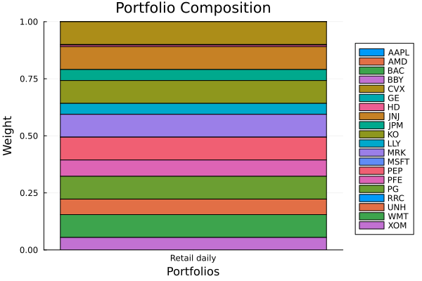

This page was generated using Literate.jl.