The source files can be found in user_guide/.
Post-processing
An optimiser returns continuous weights, which are fractions of the capital. To trade them, you need whole shares, and to show them to others, you need a report. Post-processing does both. It turns the weights into whole numbers of shares under a cash budget, and it plots the result. For more, see the post-processing examples.
using PortfolioOptimisers, CSV, TimeSeries, DataFrames, PrettyTables, Clarabel, StatsPlots, GraphRecipesresfmt = (v, i, j) -> begin return if j == 1 v else isa(v, AbstractFloat) ? "$(round(v*100, digits=3)) %" : v endend;X = TimeArray(CSV.File(joinpath(@__DIR__, "../examples/SP500.csv.gz")); timestamp = :Date)[(end - 252):end]rd = prices_to_returns(X)pr = prior(EmpiricalPrior(), rd)slv = Solver(; name = :clarabel, solver = Clarabel.Optimizer, settings = Dict("verbose" => false), check_sol = (; allow_local = true, allow_almost = true))res = optimise(MeanRisk(; obj = MinimumRisk(), opt = JuMPOptimiser(; pe = pr, slv = slv)))MeanRiskResult
jr ┼ JuMPOptimisationResult
│ pa ┼ ProcessedJuMPOptimiserAttributes
│ │ pr ┼ LowOrderPrior
│ │ │ X ┼ 252×20 Matrix{Float64}
│ │ │ o_X ┼ nothing
│ │ │ mu ┼ 20-element Vector{Float64}
│ │ │ sigma ┼ 20×20 Matrix{Float64}
│ │ │ chol ┼ nothing
│ │ │ w ┼ nothing
│ │ │ ens ┼ nothing
│ │ │ kld ┼ nothing
│ │ │ ow ┼ nothing
│ │ │ rr ┼ nothing
│ │ │ fpr ┴ nothing
│ │ wb ┼ WeightBounds
│ │ │ lb ┼ 20-element StepRangeLen{Float64, Base.TwicePrecision{Float64}, Base.TwicePrecision{Float64}, Int64}
│ │ │ ub ┴ 20-element StepRangeLen{Float64, Base.TwicePrecision{Float64}, Base.TwicePrecision{Float64}, Int64}
│ │ lt ┼ nothing
│ │ st ┼ nothing
│ │ lcsr ┼ nothing
│ │ ctr ┼ nothing
│ │ gcardr ┼ nothing
│ │ sgcardr ┼ nothing
│ │ smtx ┼ nothing
│ │ sgmtx ┼ nothing
│ │ slt ┼ nothing
│ │ sst ┼ nothing
│ │ sglt ┼ nothing
│ │ sgst ┼ nothing
│ │ tn ┼ nothing
│ │ fees ┼ nothing
│ │ plr ┼ nothing
│ │ ret ┼ ArithmeticReturn
│ │ │ settings ┼ JuMPReturnsSettings
│ │ │ │ scale ┼ Float64: 1.0
│ │ │ │ lb ┼ nothing
│ │ │ │ rte ┼ Bool: true
│ │ │ │ fee ┼ Bool: true
│ │ │ │ mic ┴ Bool: true
│ │ │ ucs ┼ nothing
│ │ │ mu ┴ 20-element Vector{Float64}
│ │ sca ┼ SumScalariser()
│ │ imsk ┴ nothing
│ retcode ┼ OptimisationSuccess
│ │ res ┴ Dict{Any, Any}: Dict{Any, Any}()
│ sol ┼ JuMPOptimisationSolution
│ │ w ┴ 20-element Vector{Float64}
│ model ┼ A JuMP Model
│ │ ├ solver: Clarabel
│ │ ├ objective_sense: MIN_SENSE
│ │ │ └ objective_function_type: QuadExpr
│ │ ├ num_variables: 21
│ │ ├ num_constraints: 4
│ │ │ ├ AffExpr in MOI.EqualTo{Float64}: 1
│ │ │ ├ Vector{AffExpr} in MOI.Nonnegatives: 1
│ │ │ ├ Vector{AffExpr} in MOI.Nonpositives: 1
│ │ │ └ Vector{AffExpr} in MOI.SecondOrderCone: 1
│ │ └ Names registered in the model
│ │ └ :G, :T, :bgt, :cdev_soc_1, :dev_1, :k, :lw, :obj_expr, :ret, :ret_1, :ret_vec, :risk, :risk_minimised, :risk_vec, :sc, :so, :variance_flag, :variance_risk_1, :w, :w_gross_ub, :w_lb, :w_ub
r ┼ Variance
│ settings ┼ RiskMeasureSettings
│ │ scale ┼ Float64: 1.0
│ │ ub ┼ nothing
│ │ rke ┴ Bool: true
│ sigma ┼ 20×20 Matrix{Float64}
│ chol ┼ nothing
│ rc ┼ nothing
│ alg ┴ SquaredSOCRiskExpr()
fb ┴ nothing
1. Finite allocation
Finite allocation turns the weights into whole numbers of shares that you can buy with a cash budget at the last prices. GreedyAllocation needs no solver. It goes through the assets from the largest target weight down, and buys as many whole shares as the target weight pays for. It then spends the cash that is left on single shares of the assets furthest below their target.
prices = vec(values(X)[end, :])cash = 100_000.0alloc = optimise(GreedyAllocation(), FiniteAllocationInput(; w = res.w, prices = prices, cash = cash))GreedyAllocationResult
retcode ┼ OptimisationSuccess
│ res ┴ nothing
shares ┼ 20-element SubArray{Float64, 1, Matrix{Float64}, Tuple{Base.Slice{Base.OneTo{Int64}}, Int64}, true}
cost ┼ 20-element SubArray{Float64, 1, Matrix{Float64}, Tuple{Base.Slice{Base.OneTo{Int64}}, Int64}, true}
w ┼ 20-element SubArray{Float64, 1, Matrix{Float64}, Tuple{Base.Slice{Base.OneTo{Int64}}, Int64}, true}
cash ┼ Float64: 14.222999999983585
fees ┼ Float64: 0.0
fb ┴ nothing
The result holds the whole shares in shares, the cost of each asset in cost, the weights after the rounding in w, and the cash that is left in cash. In the table, the realised weights are close to the target weights, and the title shows the cash that is left.
invested = sum(alloc.shares .* prices)pretty_table(DataFrame("Asset" => rd.nx, "Target weight" => res.w, "Shares" => round.(Int, alloc.shares), "Realised weight" => alloc.w); formatters = [resfmt], title = "Greedy allocation of \```math(round(Int, cash)), invested \```(round(Int, invested)), cash left \$$(round(alloc.cash, digits = 2))")Greedy allocation of ```math(round(Int, cash)), invested ```(round(Int, invested)), cash left $14.22
┌────────┬───────────────┬────────┬─────────────────┐
│ Asset │ Target weight │ Shares │ Realised weight │
│ String │ Float64 │ Int64 │ Float64 │
├────────┼───────────────┼────────┼─────────────────┤
│ AAPL │ 0.0 % │ 0 │ 0.0 % │
│ AMD │ 0.0 % │ 0 │ 0.0 % │
│ BAC │ 0.0 % │ 0 │ 0.0 % │
│ BBY │ 0.0 % │ 0 │ 0.0 % │
│ CVX │ 7.432 % │ 43 │ 7.471 % │
│ GE │ 0.806 % │ 13 │ 0.831 % │
│ HD │ 0.0 % │ 0 │ 0.0 % │
│ JNJ │ 36.974 % │ 212 │ 36.911 % │
│ JPM │ 0.749 % │ 6 │ 0.778 % │
│ KO │ 11.161 % │ 178 │ 11.146 % │
│ LLY │ 0.0 % │ 0 │ 0.0 % │
│ MRK │ 17.467 % │ 159 │ 17.426 % │
│ MSFT │ 0.0 % │ 0 │ 0.0 % │
│ PEP │ 8.978 % │ 50 │ 8.965 % │
│ PFE │ 0.0 % │ 0 │ 0.0 % │
│ PG │ 2.353 % │ 16 │ 2.386 % │
│ RRC │ 0.0 % │ 0 │ 0.0 % │
│ UNH │ 0.0 % │ 0 │ 0.0 % │
│ WMT │ 9.355 % │ 67 │ 9.393 % │
│ XOM │ 4.725 % │ 44 │ 4.692 % │
└────────┴───────────────┴────────┴─────────────────┘DiscreteAllocation solves a mixed-integer program to find an exact allocation, and it needs a Solver that handles integer variables. See the finite allocation example.
2. Reporting
plot_stacked_bar_composition plots the weights, plot_measures plots the risk against the return of a set of portfolios, plot_risk_contribution plots the risk that each asset contributes, and plot_prior plots the moments of the prior. We plot the weights of the minimum-risk portfolio.
plot_stacked_bar_composition([res], rd; xticks = (1:1, ["Min risk"]))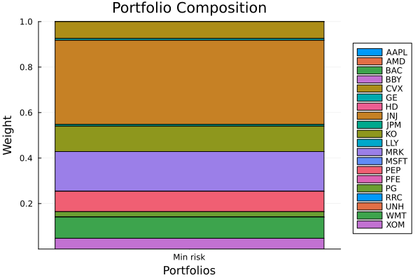
This page was generated using Literate.jl.