
The source files can be found in user_guide/.
Optimisers
This is the breadth tour of the optimiser families. Every optimiser shares the same call — optimise(estimator) (or optimise(estimator, rd) for the naive and meta ones) — and returns a result whose w field holds the asset weights. The point of this page is to show the shape of each family with one minimal call; for objectives, risk measures, variants, and trade-offs, follow the cross-links into the optimiser examples.
We fix one empirical prior and reuse it everywhere so the families are comparable.
using PortfolioOptimisers, CSV, TimeSeries, DataFrames, PrettyTables, Clarabel, StatsPlots,
      GraphRecipes

resfmt = (v, i, j) -> begin
    return if j == 1
        v
    else
        isa(v, AbstractFloat) ? "$(round(v*100, digits=3)) %" : v
    end
end;

X = TimeArray(CSV.File(joinpath(@__DIR__, "../examples/SP500.csv.gz")); timestamp = :Date)[(end - 252):end]
rd = prices_to_returns(X)
pr = prior(EmpiricalPrior(), rd)

slv = Solver(; name = :clarabel, solver = Clarabel.Optimizer,
             settings = Dict("verbose" => false),
             check_sol = (; allow_local = true, allow_almost = true))
Solver
name ┼ Symbol: :clarabel
solver ┼ UnionAll: Clarabel.MOIwrapper.Optimizer
settings ┼ Dict{String, Bool}: Dict{String, Bool}("verbose" => 0)
check_sol ┼ @NamedTuple{allow_local::Bool, allow_almost::Bool}: (allow_local = true, allow_almost = true)
add_bridges ┴ Bool: true1. Naive optimisers
Naive optimisers use simple, solver-free rules that buy robustness through unsophistication. InverseVolatility weights by the reciprocal of each asset's volatility; EqualWeighted splits capital evenly; RandomWeighted samples a Dirichlet allocation. They take the ReturnsResult directly.
res_iv = optimise(InverseVolatility(), rd)
res_ew = optimise(EqualWeighted(), rd)
NaiveOptimisationResult
pr ┼ ReturnsResult
│ nx ┼ 20-element Vector{String}
│ X ┼ 252×20 Matrix{Float64}
│ nf ┼ nothing
│ F ┼ nothing
│ nb ┼ nothing
│ B ┼ nothing
│ ts ┼ 252-element Vector{Date}
│ iv ┼ nothing
│ ivpa ┴ nothing
wb ┼ WeightBounds
│ lb ┼ 20-element StepRangeLen{Float64, Base.TwicePrecision{Float64}, Base.TwicePrecision{Float64}, Int64}
│ ub ┴ 20-element StepRangeLen{Float64, Base.TwicePrecision{Float64}, Base.TwicePrecision{Float64}, Int64}
retcode ┼ OptimisationSuccess
│ res ┴ nothing
w ┼ 20-element Vector{Float64}
fb ┴ nothing2. JuMP optimisers — MeanRisk
JuMP optimisers solve a mathematical program and are the most flexible on constraints, objectives, and risk measures. They need a JuMPOptimiser carrying the prior and a Solver (we recommend Clarabel for non-MIP problems). The workhorse is MeanRisk; its default objective is MinimumRisk.
res_mr = optimise(MeanRisk(; obj = MinimumRisk(),
                           opt = JuMPOptimiser(; pe = pr, slv = slv)))
MeanRiskResult
jr ┼ JuMPOptimisationResult
│ pa ┼ ProcessedJuMPOptimiserAttributes
│ │ pr ┼ LowOrderPrior
│ │ │ X ┼ 252×20 Matrix{Float64}
│ │ │ mu ┼ 20-element Vector{Float64}
│ │ │ sigma ┼ 20×20 Matrix{Float64}
│ │ │ chol ┼ nothing
│ │ │ w ┼ nothing
│ │ │ ens ┼ nothing
│ │ │ kld ┼ nothing
│ │ │ ow ┼ nothing
│ │ │ rr ┼ nothing
│ │ │ f_mu ┼ nothing
│ │ │ f_sigma ┼ nothing
│ │ │ f_w ┴ nothing
│ │ wb ┼ WeightBounds
│ │ │ lb ┼ 20-element StepRangeLen{Float64, Base.TwicePrecision{Float64}, Base.TwicePrecision{Float64}, Int64}
│ │ │ ub ┴ 20-element StepRangeLen{Float64, Base.TwicePrecision{Float64}, Base.TwicePrecision{Float64}, Int64}
│ │ lt ┼ nothing
│ │ st ┼ nothing
│ │ lcsr ┼ nothing
│ │ ctr ┼ nothing
│ │ gcardr ┼ nothing
│ │ sgcardr ┼ nothing
│ │ smtx ┼ nothing
│ │ sgmtx ┼ nothing
│ │ slt ┼ nothing
│ │ sst ┼ nothing
│ │ sglt ┼ nothing
│ │ sgst ┼ nothing
│ │ tn ┼ nothing
│ │ fees ┼ nothing
│ │ plr ┼ nothing
│ │ ret ┼ ArithmeticReturn
│ │ │ ucs ┼ nothing
│ │ │ lb ┼ nothing
│ │ │ mu ┴ 20-element Vector{Float64}
│ retcode ┼ OptimisationSuccess
│ │ res ┴ Dict{Any, Any}: Dict{Any, Any}()
│ sol ┼ JuMPOptimisationSolution
│ │ w ┴ 20-element Vector{Float64}
│ model ┼ A JuMP Model
│ │ ├ solver: Clarabel
│ │ ├ objective_sense: MIN_SENSE
│ │ │ └ objective_function_type: QuadExpr
│ │ ├ num_variables: 21
│ │ ├ num_constraints: 4
│ │ │ ├ AffExpr in MOI.EqualTo{Float64}: 1
│ │ │ ├ Vector{AffExpr} in MOI.Nonnegatives: 1
│ │ │ ├ Vector{AffExpr} in MOI.Nonpositives: 1
│ │ │ └ Vector{AffExpr} in MOI.SecondOrderCone: 1
│ │ └ Names registered in the model
│ │ └ :G, :bgt, :dev_1, :dev_1_soc, :k, :lw, :obj_expr, :ret, :risk, :risk_vec, :sc, :so, :variance_flag, :variance_risk_1, :w, :w_lb, :w_ub
fb ┴ nothingMeanRisk also offers MaximumUtility, MaximumRatio and MaximumReturn objectives and efficient frontiers — see MeanRisk Objectives and Efficient Frontier.
The risk measure is the r field (of MeanRisk and of the clustering optimisers below); the default is Variance. Which family you pick encodes what kind of risk you penalise:
Moment-based —
Variance,StandardDeviation, and higher-moment measures. Cheap and classic; the right default when returns are roughly symmetric and you care about overall dispersion.Quantile / tail —
ConditionalValueatRisk,EntropicValueatRisk,RelativisticValueatRisk, … Reach for these when the left tail matters more than overall spread (Exotic Tail Risk Measures).OWA (ordered-weight) —
OrderedWeightsArraymeasures weight the whole ordered loss distribution, the most general family (OWA Risk Measures).
You can mix several in one objective (Multiple Risk Measures). Drawdown measures (MaximumDrawdown, ConditionalDrawdownatRisk, …) penalise peak-to-trough paths (Drawdown Risk Measures); the same drawdown notion is also useful purely as a post-optimisation diagnostic — via drawdowns on a realised book — when you want to measure rather than optimise it (Performance Attribution).
The other JuMP families follow the same opt = JuMPOptimiser(...) pattern:
RiskBudgeting/RelaxedRiskBudgeting— target a risk contribution per asset or factor (Risk Budgeting).NearOptimalCentering— a robust point near the efficient frontier (Near Optimal Centering).
Here is the minimal risk-budgeting call (equal risk contribution by default):
res_rb = optimise(RiskBudgeting(; opt = JuMPOptimiser(; pe = pr, slv = slv)))RiskBudgetingResult
jr ┼ JuMPOptimisationResult
│ pa ┼ ProcessedJuMPOptimiserAttributes
│ │ pr ┼ LowOrderPrior
│ │ │ X ┼ 252×20 Matrix{Float64}
│ │ │ mu ┼ 20-element Vector{Float64}
│ │ │ sigma ┼ 20×20 Matrix{Float64}
│ │ │ chol ┼ nothing
│ │ │ w ┼ nothing
│ │ │ ens ┼ nothing
│ │ │ kld ┼ nothing
│ │ │ ow ┼ nothing
│ │ │ rr ┼ nothing
│ │ │ f_mu ┼ nothing
│ │ │ f_sigma ┼ nothing
│ │ │ f_w ┴ nothing
│ │ wb ┼ WeightBounds
│ │ │ lb ┼ 20-element StepRangeLen{Float64, Base.TwicePrecision{Float64}, Base.TwicePrecision{Float64}, Int64}
│ │ │ ub ┴ 20-element StepRangeLen{Float64, Base.TwicePrecision{Float64}, Base.TwicePrecision{Float64}, Int64}
│ │ lt ┼ nothing
│ │ st ┼ nothing
│ │ lcsr ┼ nothing
│ │ ctr ┼ nothing
│ │ gcardr ┼ nothing
│ │ sgcardr ┼ nothing
│ │ smtx ┼ nothing
│ │ sgmtx ┼ nothing
│ │ slt ┼ nothing
│ │ sst ┼ nothing
│ │ sglt ┼ nothing
│ │ sgst ┼ nothing
│ │ tn ┼ nothing
│ │ fees ┼ nothing
│ │ plr ┼ nothing
│ │ ret ┼ ArithmeticReturn
│ │ │ ucs ┼ nothing
│ │ │ lb ┼ nothing
│ │ │ mu ┴ 20-element Vector{Float64}
│ retcode ┼ OptimisationSuccess
│ │ res ┴ Dict{Any, Any}: Dict{Any, Any}()
│ sol ┼ JuMPOptimisationSolution
│ │ w ┴ 20-element Vector{Float64}
│ model ┼ A JuMP Model
│ │ ├ solver: Clarabel
│ │ ├ objective_sense: MIN_SENSE
│ │ │ └ objective_function_type: QuadExpr
│ │ ├ num_variables: 42
│ │ ├ num_constraints: 25
│ │ │ ├ AffExpr in MOI.EqualTo{Float64}: 1
│ │ │ ├ AffExpr in MOI.GreaterThan{Float64}: 1
│ │ │ ├ Vector{AffExpr} in MOI.Nonnegatives: 1
│ │ │ ├ Vector{AffExpr} in MOI.Nonpositives: 1
│ │ │ ├ Vector{AffExpr} in MOI.SecondOrderCone: 1
│ │ │ └ Vector{AffExpr} in MOI.ExponentialCone: 20
│ │ └ Names registered in the model
│ │ └ :G, :bgt, :clog_w, :crkb, :dev_1, :dev_1_soc, :k, :log_w, :lw, :obj_expr, :ret, :risk, :risk_vec, :sc, :so, :variance_flag, :variance_risk_1, :w, :w_lb, :w_ub
prb ┼ ProcessedAssetRiskBudgetingAttributes
│ rkb ┼ RiskBudget
│ │ val ┴ 20-element StepRangeLen{Float64, Base.TwicePrecision{Float64}, Base.TwicePrecision{Float64}, Int64}
fb ┴ nothingWhich risk measures each optimiser family accepts
Compatibility is a property of the optimiser family, not the individual optimiser: every JuMP optimiser accepts the same RiskMeasures, and clustering optimisers additionally accept the hierarchical-only measures. You can ask programmatically with supports_risk_measure / supported_risk_measures:
supports_risk_measure(MeanRisk, ConditionalValueatRisk)   # true
supported_risk_measures(HierarchicalRiskParity)           # OptimisationRiskMeasure
The table below is generated from that same predicate, so it can never drift from what the optimisers actually dispatch on. Meta-optimisers (NestedClustered, Stacking, SubsetResampling) are omitted because their acceptance is instance-specific: they delegate, accepting a measure only when every constituent optimiser does (the intersection of their children's categories).
using InteractiveUtils
# Leaf risk-measure types (concrete or parametric) under a supertype.
function _leaf_risk_measures(T, acc = Type[])
    subs = subtypes(T)
    if isempty(subs)
        push!(acc, T)
    else
        for S in subs
            _leaf_risk_measures(S, acc)
        end
    end
    return acc
end
rms = sort(unique(vcat(_leaf_risk_measures(RiskMeasure),
                       _leaf_risk_measures(HierarchicalRiskMeasure))); by = nameof)
tick(x) = x ? "✓" : ""
pretty_table(DataFrame("Risk measure" => String.(nameof.(rms)),
                       "JuMP (MeanRisk, RiskBudgeting, NOC, FRC)" =>
                           [tick(supports_risk_measure(MeanRisk, M)) for M in rms],
                       "Clustering (HRP, HERC, SCHRP)" =>
                           [tick(supports_risk_measure(HierarchicalRiskParity, M))
                            for M in rms]))
┌───────────────────────────────────────────────────┬───────────────────────────
│ Risk measure │ JuMP (MeanRisk, RiskBudg ⋯
│ String │ ⋯
├───────────────────────────────────────────────────┼───────────────────────────
│ AverageDrawdown │ ⋯
│ BrownianDistanceVariance │ ⋯
│ ConditionalDrawdownatRisk │ ⋯
│ ConditionalValueatRisk │ ⋯
│ ConditionalValueatRiskRange │ ⋯
│ DistributionallyRobustConditionalDrawdownatRisk │ ⋯
│ DistributionallyRobustConditionalValueatRisk │ ⋯
│ DistributionallyRobustConditionalValueatRiskRange │ ⋯
│ DrawdownatRisk │ ⋯
│ EntropicDrawdownatRisk │ ⋯
│ EntropicValueatRisk │ ⋯
│ EntropicValueatRiskRange │ ⋯
│ EqualRisk │ ⋯
│ GenericValueatRiskRange │ ⋯
│ HighOrderMoment │ ⋯
│ ⋮ │ ⋱
└───────────────────────────────────────────────────┴───────────────────────────
2 columns and 34 rows omitted3. Clustering optimisers
Clustering optimisers build the allocation from the asset correlation hierarchy instead of a single program. They take a HierarchicalOptimiser carrying the prior and a clustering estimate. HierarchicalRiskParity (HRP) is the canonical one; HierarchicalEqualRiskContribution and SchurComplementHierarchicalRiskParity are its siblings — see Clustering Optimisers.
clr = clusterise(ClustersEstimator(), pr.X)
hopt = HierarchicalOptimiser(; pe = pr, cle = clr)
res_hrp = optimise(HierarchicalRiskParity(; opt = hopt, r = Variance()))
HierarchicalResult
pr ┼ LowOrderPrior
│ X ┼ 252×20 Matrix{Float64}
│ mu ┼ 20-element Vector{Float64}
│ sigma ┼ 20×20 Matrix{Float64}
│ chol ┼ nothing
│ w ┼ nothing
│ ens ┼ nothing
│ kld ┼ nothing
│ ow ┼ nothing
│ rr ┼ nothing
│ f_mu ┼ nothing
│ f_sigma ┼ nothing
│ f_w ┴ nothing
clr ┼ Clusters
│ res ┼ Clustering.Hclust{Float64}([-1 -13; -2 1; … ; 15 16; 18 17], [0.2992796916890263, 0.3905612031361099, 0.4116454947407609, 0.22529867864314176, 0.48924055164900887, 0.28518628966607656, 0.38008631653392483, 0.58425801808901, 0.4209146698909511, 0.4605479608276049, 0.491265779899127, 0.5080236207888611, 0.6028393326616824, 0.24670816017739164, 0.5174631833197462, 0.6821605083740293, 0.739945604975504, 0.9602133336085281, 1.0707389175241802], [5, 20, 17, 3, 9, 6, 2, 1, 13, 7, 4, 19, 14, 10, 16, 18, 11, 8, 12, 15], :ward)
│ S ┼ 20×20 Matrix{Float64}
│ D ┼ 20×20 Matrix{Float64}
│ P ┼ nothing
│ k ┴ Int64: 2
wb ┼ WeightBounds
│ lb ┼ 20-element StepRangeLen{Float64, Base.TwicePrecision{Float64}, Base.TwicePrecision{Float64}, Int64}
│ ub ┴ 20-element StepRangeLen{Float64, Base.TwicePrecision{Float64}, Base.TwicePrecision{Float64}, Int64}
fees ┼ nothing
retcode ┼ OptimisationSuccess
│ res ┴ nothing
w ┼ 20-element Vector{Float64}
fb ┴ nothing4. Meta-optimisers
Meta-optimisers compose other optimisers. NestedClustered (NCO) runs an inner optimiser within each cluster and an outer optimiser across the cluster representatives; Stacking and SubsetResampling blend several fits — see Meta Optimisers. The inner optimiser carries the prior; the outer one does not.
res_nco = optimise(NestedClustered(; pe = pr, cle = clr,
                                   opti = MeanRisk(; obj = MinimumRisk(),
                                                   opt = JuMPOptimiser(; pe = pr,
                                                                       slv = slv)),
                                   opto = MeanRisk(; obj = MinimumRisk(),
                                                   opt = JuMPOptimiser(; slv = slv))), rd)
NestedClusteredResult
pr ┼ LowOrderPrior
│ X ┼ 252×20 Matrix{Float64}
│ mu ┼ 20-element Vector{Float64}
│ sigma ┼ 20×20 Matrix{Float64}
│ chol ┼ nothing
│ w ┼ nothing
│ ens ┼ nothing
│ kld ┼ nothing
│ ow ┼ nothing
│ rr ┼ nothing
│ f_mu ┼ nothing
│ f_sigma ┼ nothing
│ f_w ┴ nothing
clr ┼ Clusters
│ res ┼ Clustering.Hclust{Float64}([-1 -13; -2 1; … ; 15 16; 18 17], [0.2992796916890263, 0.3905612031361099, 0.4116454947407609, 0.22529867864314176, 0.48924055164900887, 0.28518628966607656, 0.38008631653392483, 0.58425801808901, 0.4209146698909511, 0.4605479608276049, 0.491265779899127, 0.5080236207888611, 0.6028393326616824, 0.24670816017739164, 0.5174631833197462, 0.6821605083740293, 0.739945604975504, 0.9602133336085281, 1.0707389175241802], [5, 20, 17, 3, 9, 6, 2, 1, 13, 7, 4, 19, 14, 10, 16, 18, 11, 8, 12, 15], :ward)
│ S ┼ 20×20 Matrix{Float64}
│ D ┼ 20×20 Matrix{Float64}
│ P ┼ nothing
│ k ┴ Int64: 2
wb ┼ WeightBounds
│ lb ┼ Vector{Float64}: [-Inf, -Inf]
│ ub ┴ Vector{Float64}: [Inf, Inf]
fees ┼ nothing
resi ┼ 2-element Vector{MeanRiskResult}
│ MeanRiskResult ⋯
│ MeanRiskResult ⋯
reso ┼ MeanRiskResult
│ jr ┼ JuMPOptimisationResult
│ │ pa ┼ ProcessedJuMPOptimiserAttributes
│ │ │ pr ┼ LowOrderPrior
│ │ │ │ X ┼ 252×2 Matrix{Float64}
│ │ │ │ mu ┼ Vector{Float64}: [0.000363546280760209, 0.0006527974205718796]
│ │ │ │ sigma ┼ 2×2 Matrix{Float64}
│ │ │ │ chol ┼ nothing
│ │ │ │ w ┼ nothing
│ │ │ │ ens ┼ nothing
│ │ │ │ kld ┼ nothing
│ │ │ │ ow ┼ nothing
│ │ │ │ rr ┼ nothing
│ │ │ │ f_mu ┼ nothing
│ │ │ │ f_sigma ┼ nothing
│ │ │ │ f_w ┴ nothing
│ │ │ wb ┼ WeightBounds
│ │ │ │ lb ┼ StepRangeLen{Float64, Base.TwicePrecision{Float64}, Base.TwicePrecision{Float64}, Int64}: StepRangeLen(0.0, 0.0, 2)
│ │ │ │ ub ┴ StepRangeLen{Float64, Base.TwicePrecision{Float64}, Base.TwicePrecision{Float64}, Int64}: StepRangeLen(1.0, 0.0, 2)
│ │ │ lt ┼ nothing
│ │ │ st ┼ nothing
│ │ │ lcsr ┼ nothing
│ │ │ ctr ┼ nothing
│ │ │ gcardr ┼ nothing
│ │ │ sgcardr ┼ nothing
│ │ │ smtx ┼ nothing
│ │ │ sgmtx ┼ nothing
│ │ │ slt ┼ nothing
│ │ │ sst ┼ nothing
│ │ │ sglt ┼ nothing
│ │ │ sgst ┼ nothing
│ │ │ tn ┼ nothing
│ │ │ fees ┼ nothing
│ │ │ plr ┼ nothing
│ │ │ ret ┼ ArithmeticReturn
│ │ │ │ ucs ┼ nothing
│ │ │ │ lb ┼ nothing
│ │ │ │ mu ┴ Vector{Float64}: [0.000363546280760209, 0.0006527974205718796]
│ │ retcode ┼ OptimisationSuccess
│ │ │ res ┴ Dict{Any, Any}: Dict{Any, Any}()
│ │ sol ┼ JuMPOptimisationSolution
│ │ │ w ┴ Vector{Float64}: [0.13998673390975952, 0.8600132660902406]
│ │ model ┼ A JuMP Model
│ │ │ ├ solver: Clarabel
│ │ │ ├ objective_sense: MIN_SENSE
│ │ │ │ └ objective_function_type: QuadExpr
│ │ │ ├ num_variables: 3
│ │ │ ├ num_constraints: 4
│ │ │ │ ├ AffExpr in MOI.EqualTo{Float64}: 1
│ │ │ │ ├ Vector{AffExpr} in MOI.Nonnegatives: 1
│ │ │ │ ├ Vector{AffExpr} in MOI.Nonpositives: 1
│ │ │ │ └ Vector{AffExpr} in MOI.SecondOrderCone: 1
│ │ │ └ Names registered in the model
│ │ │ └ :G, :bgt, :dev_1, :dev_1_soc, :k, :lw, :obj_expr, :ret, :risk, :risk_vec, :sc, :so, :variance_flag, :variance_risk_1, :w, :w_lb, :w_ub
│ fb ┴ nothing
cv ┼ nothing
retcode ┼ OptimisationSuccess
│ res ┴ nothing
w ┼ 20-element Vector{Float64}
fb ┴ nothing5. Comparing the families
One prior, six optimisers, six allocations. The naive rules, risk budgeting, and the clustering hierarchy spread weight broadly (max weight in single digits to low teens); MeanRisk(MinimumRisk) and NCO concentrate into a few low-variance names (max weight ≈ a third). Same data, very different portfolios — which is the point of having a menu.
results = [res_iv, res_ew, res_mr, res_rb, res_hrp, res_nco]
labels = ["InvVol", "EqualW", "MinRisk", "RiskBudget", "HRP", "NCO"]

pretty_table(DataFrame(["Asset" => rd.nx,
                        [labels[i] => results[i].w for i in eachindex(results)]...]);
             formatters = [resfmt], title = "Weights by optimiser family")

plot_stacked_bar_composition(results, rd; xticks = (1:length(labels), labels))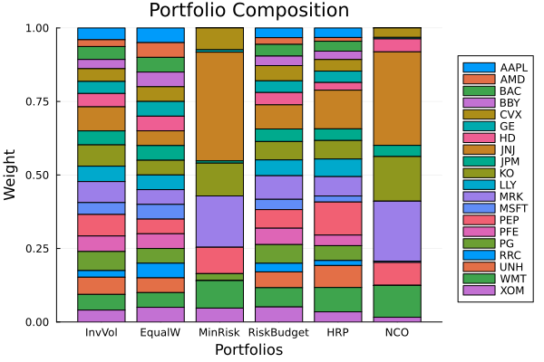
This page was generated using Literate.jl.