
The source files can be found in examples/.
Advanced Black–Litterman variants
The base BlackLittermanPrior (previous page) works entirely in asset space: views are statements about individual assets or asset groups. But views are often more naturally expressed about factors — "momentum will earn a premium", "quality minus low-volatility will be negative" — and sometimes you hold asset and factor views at once. PortfolioOptimisers ships three variants of the model for exactly these cases:
BayesianBlackLittermanPrior— the Bayesian formulation that sits on top of aFactorPrior. Views are expressed on the factors, and the factor structure propagates the posterior back to the assets.FactorBlackLittermanPrior— expresses views directly on factor premia and pushes them to the assets through a factor regression. Thersdflag controls whether idiosyncratic residual variance is retained, andlis the risk-aversion of the implied factor equilibrium.AugmentedBlackLittermanPrior— carries both asset views (a_views) and factor views (f_views) simultaneously, each with its own asset set and confidence.
All three return an asset-space posterior (mu, sigma) you can feed to any optimiser, exactly like the base model.
When to reach for this
Reach for these when your conviction is about factors rather than (or in addition to) individual names: a macro view on momentum or value, a quality-vs-low-vol spread, or a desk that wants to combine a stock-level call with a factor-level call in one coherent posterior. If all your views are plain asset statements, the base BlackLittermanPrior is simpler and enough.
Factor data required
These variants need factor returns, so the ReturnsResult must be built with a factor block via prices_to_returns(X, F). Factor views and factor sets refer to the factor names in rd.nf.
using PortfolioOptimisers, PrettyTables, DataFrames

mmtfmt = (v, i, j) -> begin
    if j == 1
        return v
    else
        return isa(v, Number) ? "$(round(v * 100, digits = 4)) %" : v
    end
end;
resfmt = (v, i, j) -> begin
    if j == 1
        return v
    else
        return isa(v, Number) ? "$(round(v * 100, digits = 3)) %" : v
    end
end;
1. Data, sets, and the equilibrium baseline
We load the S&P 500 slice with its factor block, then declare two AssetSets: one over the assets (with a couple of groups, for the augmented asset views) and one over the factor names. The EquilibriumExpectedReturns prior is the neutral anchor every Black–Litterman posterior tilts away from.
using CSV, TimeSeries

X = TimeArray(CSV.File(joinpath(@__DIR__, "..", "SP500.csv.gz")); timestamp = :Date)[(end - 252):end]
F = TimeArray(CSV.File(joinpath(@__DIR__, "..", "Factors.csv.gz")); timestamp = :Date)[(end - 252):end]
rd = prices_to_returns(X, F)

asset_sets = AssetSets(;
                       dict = Dict("nx" => rd.nx, "tech" => ["AAPL", "AMD", "MSFT"],
                                   "energy" => ["CVX"]))
factor_sets = AssetSets(; dict = Dict("nx" => rd.nf))
tau = 1 / size(rd.X, 1)

pr_eq = prior(EmpiricalPrior(; me = EquilibriumExpectedReturns()), rd)
LowOrderPrior
X ┼ 252×20 Matrix{Float64}
mu ┼ 20-element Vector{Float64}
sigma ┼ 20×20 Matrix{Float64}
chol ┼ nothing
w ┼ nothing
ens ┼ nothing
kld ┼ nothing
ow ┼ nothing
rr ┼ nothing
f_mu ┼ nothing
f_sigma ┼ nothing
f_w ┴ nothingThe factors available in this dataset:
pretty_table(DataFrame(; factor = rd.nf); title = "Factor names (rd.nf)")Factor names (rd.nf)
┌────────┐
│ factor │
│ String │
├────────┤
│ MTUM │
│ QUAL │
│ SIZE │
│ USMV │
│ VLUE │
└────────┘2. Bayesian Black–Litterman: factor views on a factor prior
BayesianBlackLittermanPrior takes a FactorPrior as its base estimator and accepts views written in factor space (so its sets are the factor sets). It is the Bayesian formulation: the factor prior supplies the structure, the views update the factor means, and the result is mapped back to an asset-space posterior.
Our factor views: momentum earns 5 bps/day, and quality underperforms low-volatility by 3 bps/day.
factor_views = LinearConstraintEstimator(;
                                         val = ["MTUM == 0.0005", "QUAL - USMV == -0.0003"])

pr_bayes = prior(BayesianBlackLittermanPrior(; pe = FactorPrior(; pe = EmpiricalPrior()),
                                             sets = factor_sets, tau = tau,
                                             views = factor_views), rd)
LowOrderPrior
X ┼ 252×20 Matrix{Float64}
mu ┼ 20-element Vector{Float64}
sigma ┼ 20×20 Matrix{Float64}
chol ┼ nothing
w ┼ nothing
ens ┼ nothing
kld ┼ nothing
ow ┼ nothing
rr ┼ Regression
│ M ┼ 20×5 SubArray{Float64, 2, Matrix{Float64}, Tuple{Base.Slice{Base.OneTo{Int64}}, UnitRange{Int64}}, true}
│ L ┼ 20×5 SubArray{Float64, 2, Matrix{Float64}, Tuple{Base.Slice{Base.OneTo{Int64}}, UnitRange{Int64}}, true}
│ b ┴ 20-element SubArray{Float64, 1, Matrix{Float64}, Tuple{Base.Slice{Base.OneTo{Int64}}, Int64}, true}
f_mu ┼ Vector{Float64}: [-0.0007221367902182355, -0.0008384535501032073, -0.0006253517821839465, -0.0003358529620217417, -0.000559091885073412]
f_sigma ┼ 5×5 Matrix{Float64}
f_w ┴ nothing3. Factor Black–Litterman: views on factor premia
FactorBlackLittermanPrior also takes factor views, but propagates them to the assets through the factor regression rather than a factor prior. Two knobs matter:
rsd— keep the idiosyncratic residual variance (true) or drop it (false), i.e. whether the posterior covariance is the full asset covariance or only its factor-explained part.l— the risk-aversion of the implied factor equilibrium.
We build both rsd settings and a higher-risk-aversion variant to show each knob moves the posterior.
pr_fbl_rsd = prior(FactorBlackLittermanPrior(; pe = EmpiricalPrior(), rsd = true,
                                             sets = factor_sets, tau = tau,
                                             views = factor_views), rd)
pr_fbl_nors = prior(FactorBlackLittermanPrior(; pe = EmpiricalPrior(), rsd = false,
                                              sets = factor_sets, tau = tau,
                                              views = factor_views), rd)
pr_fbl_l = prior(FactorBlackLittermanPrior(; pe = EmpiricalPrior(), rsd = true, l = 5.0,
                                           sets = factor_sets, tau = tau,
                                           views = factor_views), rd)

i_aapl = findfirst(==("AAPL"), rd.nx)
pretty_table(DataFrame(; quantity = ["AAPL posterior mean", "AAPL posterior variance"],
                       rsd_true = [pr_fbl_rsd.mu[i_aapl], pr_fbl_rsd.sigma[i_aapl, i_aapl]],
                       rsd_false = [pr_fbl_nors.mu[i_aapl],
                                    pr_fbl_nors.sigma[i_aapl, i_aapl]]);
             formatters = [mmtfmt], title = "Factor BL: residual variance on vs off")
Factor BL: residual variance on vs off
┌─────────────────────────┬──────────┬───────────┐
│ quantity │ rsd_true │ rsd_false │
│ String │ Float64 │ Float64 │
├─────────────────────────┼──────────┼───────────┤
│ AAPL posterior mean │ -0.044 % │ -0.044 % │
│ AAPL posterior variance │ 0.0501 % │ 0.0384 % │
└─────────────────────────┴──────────┴───────────┘Dropping the residual variance (rsd = false) leaves only the factor-explained part of the covariance, so the posterior variance is smaller — the model trusts the factor structure to explain all risk.
4. Augmented Black–Litterman: asset and factor views together
AugmentedBlackLittermanPrior is the most general: it takes asset views (a_views, with asset sets) and factor views (f_views, with factor sets) in the same posterior. Use it when you have a stock-specific call and a factor call you do not want to choose between.
asset_views = LinearConstraintEstimator(; val = ["AAPL == 0.0008", "tech == 0.0006"])

pr_aug = prior(AugmentedBlackLittermanPrior(; a_sets = asset_sets, f_sets = factor_sets,
                                            tau = tau, a_views = asset_views,
                                            f_views = factor_views), rd)
LowOrderPrior
X ┼ 252×20 Matrix{Float64}
mu ┼ 20-element Vector{Float64}
sigma ┼ 20×20 Matrix{Float64}
chol ┼ nothing
w ┼ nothing
ens ┼ nothing
kld ┼ nothing
ow ┼ nothing
rr ┼ Regression
│ M ┼ 20×5 SubArray{Float64, 2, Matrix{Float64}, Tuple{Base.Slice{Base.OneTo{Int64}}, UnitRange{Int64}}, true}
│ L ┼ 20×5 SubArray{Float64, 2, Matrix{Float64}, Tuple{Base.Slice{Base.OneTo{Int64}}, UnitRange{Int64}}, true}
│ b ┴ 20-element SubArray{Float64, 1, Matrix{Float64}, Tuple{Base.Slice{Base.OneTo{Int64}}, Int64}, true}
f_mu ┼ Vector{Float64}: [-0.0007221367902182355, -0.0008384535501032073, -0.0006253517821839465, -0.0003358529620217417, -0.000559091885073412]
f_sigma ┼ 5×5 Matrix{Float64}
f_w ┴ nothing5. Comparing the posteriors
Each variant produces a different asset-space posterior mean. Below we line them up against the equilibrium anchor for the first few assets — the factor views move the whole cross-section, and the augmented model additionally tilts the assets named in its asset views.
cmp = DataFrame(; Assets = rd.nx, Equilibrium = pr_eq.mu, Bayesian = pr_bayes.mu,
                Factor = pr_fbl_rsd.mu, Augmented = pr_aug.mu)
pretty_table(first(cmp, 8); formatters = [mmtfmt],
             title = "Posterior expected returns (first 8 assets)")

using StatsPlots, GraphRecipes
plot_mu(pr_aug, rd.nx)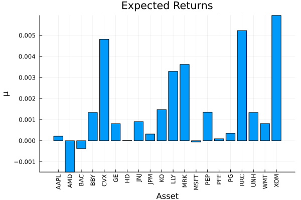
6. From views to portfolios
The payoff is the same as for the base model: each posterior reshapes the optimal portfolio. We solve a maximum-ratio portfolio under the equilibrium prior and under each variant, then compare the compositions.
using Clarabel

slv = Solver(; name = :clarabel1, solver = Clarabel.Optimizer,
             settings = Dict("verbose" => false),
             check_sol = (; allow_local = true, allow_almost = true))
rf = 4.2 / 100 / 252

priors = ["Equilibrium" => pr_eq, "Bayesian" => pr_bayes, "Factor" => pr_fbl_rsd,
          "Augmented" => pr_aug]
res = [optimise(MeanRisk(; obj = MaximumRatio(; rf = rf),
                         opt = JuMPOptimiser(; pe = p, slv = slv))) for (_, p) in priors]

pretty_table(DataFrame(hcat(rd.nx, [r.w for r in res]...),
                       [:assets; Symbol.(first.(priors))...]); formatters = [resfmt],
             title = "Maximum-ratio weights by prior")

plot_stacked_bar_composition(res, rd; xticks = (1:length(priors), first.(priors)))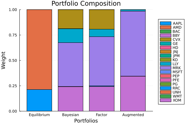
Summary
The Black–Litterman family extends well past asset-space views:
BayesianBlackLittermanPriorplaces factor views on aFactorPrior.FactorBlackLittermanPriorpropagates factor-premia views through a regression, withrsdcontrolling residual variance andlthe implied equilibrium risk-aversion.AugmentedBlackLittermanPriorblends asset views and factor views in one posterior.
All three return a standard asset-space posterior, so they drop into any optimiser exactly like the base model — the difference is only in where the views live.
This page was generated using Literate.jl.