
The source files can be found in examples/.
Higher moment estimation
Mean–variance optimisation only looks at the first two moments. But asset returns are skewed and fat-tailed, and risk measures like NegativeSkewness and Kurtosis need estimates of the coskewness and cokurtosis tensors to capture that. These high-order moments are even harder to estimate than the covariance: the cokurtosis matrix is
In PortfolioOptimisers the high-order moments live in a HighOrderPriorEstimator, which wraps a low-order prior and adds a Coskewness (ske) and Cokurtosis (kte) estimator. Each accepts the same MatrixProcessing pipeline — Denoise and LoGo — that we apply to covariances.
When to reach for this
Reach for high-order moment estimation whenever you optimise against a skew- or tail-sensitive risk measure (NegativeSkewness, Kurtosis, and the square-root variants), or build a Pareto surface over them. And reach for denoised high-order moments essentially always when you do: the raw cokurtosis on a short window is numerically singular, so denoising is what makes these optimisations well-posed rather than a nicety. If you only use variance/tail measures that need no tensors, skip it.
using PortfolioOptimisers, PrettyTables, LinearAlgebra

hmmtfmt = (v, i, j) -> begin
    if j == 1
        return v
    else
        return isa(v, Number) ? "$(round(v, digits=6))" : v
    end
end;
resfmt = (v, i, j) -> begin
    if j == 1
        return v
    else
        return isa(v, Number) ? "$(round(v*100, digits=3)) %" : v
    end
end;
1. ReturnsResult data
We use the same S&P 500 slice as the other examples.
using CSV, TimeSeries, DataFrames

X = TimeArray(CSV.File(joinpath(@__DIR__, "..", "SP500.csv.gz")); timestamp = :Date)[(end - 252):end]
rd = prices_to_returns(X)
ReturnsResult
nx ┼ 20-element Vector{String}
X ┼ 252×20 Matrix{Float64}
nf ┼ nothing
F ┼ nothing
nb ┼ nothing
B ┼ nothing
ts ┼ 252-element Vector{Date}
iv ┼ nothing
ivpa ┴ nothing2. High-order priors
We build three high-order priors that differ only in how the coskewness and cokurtosis are processed: raw (vanilla), FixedDenoised, and LoGo-sparsified. We then compare the condition numbers of the coskewness negative-spectral-slice matrix V and the cokurtosis matrix kt.
hopes = ["Vanilla" => HighOrderPriorEstimator(),
         "Denoise" => HighOrderPriorEstimator(;
                                              ske = Coskewness(;
                                                               mp = MatrixProcessing(;
                                                                                     dn = Denoise(;
                                                                                                  alg = FixedDenoise()))),
                                              kte = Cokurtosis(;
                                                               mp = MatrixProcessing(;
                                                                                     dn = Denoise(;
                                                                                                  alg = FixedDenoise())))),
         "LoGo" => HighOrderPriorEstimator(;
                                           ske = Coskewness(;
                                                            mp = MatrixProcessing(;
                                                                                  dn = Denoise(),
                                                                                  alg = LoGo())),
                                           kte = Cokurtosis(;
                                                            mp = MatrixProcessing(;
                                                                                  dn = Denoise(),
                                                                                  alg = LoGo())))]

prs = [k => prior(pe, rd) for (k, pe) in hopes]
3-element Vector{Pair{String}}:
"Vanilla" => HighOrderPrior
pr ┼ LowOrderPrior
│ X ┼ 252×20 Matrix{Float64}
│ mu ┼ 20-element Vector{Float64}
│ sigma ┼ 20×20 Matrix{Float64}
│ chol ┼ nothing
│ w ┼ nothing
│ ens ┼ nothing
│ kld ┼ nothing
│ ow ┼ nothing
│ rr ┼ nothing
│ f_mu ┼ nothing
│ f_sigma ┼ nothing
│ f_w ┴ nothing
kt ┼ 400×400 Matrix{Float64}
D2 ┼ 400×210 SparseArrays.SparseMatrixCSC{Int64, Int64}
L2 ┼ 210×400 SparseArrays.SparseMatrixCSC{Int64, Int64}
S2 ┼ 210×400 SparseArrays.SparseMatrixCSC{Int64, Int64}
sk ┼ 20×400 Matrix{Float64}
V ┼ 20×20 Matrix{Float64}
skmp ┼ MatrixProcessing
│ pdm ┼ Posdef
│ │ alg ┼ UnionAll: NearestCorrelationMatrix.Newton
│ │ kwargs ┴ @NamedTuple{}: NamedTuple()
│ dn ┼ nothing
│ dt ┼ nothing
│ alg ┼ nothing
│ order ┴ NTuple{4, Symbol}: (:pdm, :dn, :dt, :alg)
f_kt ┼ nothing
f_sk ┼ nothing
f_V ┴ nothing
"Denoise" => HighOrderPrior
pr ┼ LowOrderPrior
│ X ┼ 252×20 Matrix{Float64}
│ mu ┼ 20-element Vector{Float64}
│ sigma ┼ 20×20 Matrix{Float64}
│ chol ┼ nothing
│ w ┼ nothing
│ ens ┼ nothing
│ kld ┼ nothing
│ ow ┼ nothing
│ rr ┼ nothing
│ f_mu ┼ nothing
│ f_sigma ┼ nothing
│ f_w ┴ nothing
kt ┼ 400×400 Matrix{Float64}
D2 ┼ 400×210 SparseArrays.SparseMatrixCSC{Int64, Int64}
L2 ┼ 210×400 SparseArrays.SparseMatrixCSC{Int64, Int64}
S2 ┼ 210×400 SparseArrays.SparseMatrixCSC{Int64, Int64}
sk ┼ 20×400 Matrix{Float64}
V ┼ 20×20 Matrix{Float64}
skmp ┼ MatrixProcessing
│ pdm ┼ Posdef
│ │ alg ┼ UnionAll: NearestCorrelationMatrix.Newton
│ │ kwargs ┴ @NamedTuple{}: NamedTuple()
│ dn ┼ Denoise
│ │ pdm ┼ Posdef
│ │ │ alg ┼ UnionAll: NearestCorrelationMatrix.Newton
│ │ │ kwargs ┴ @NamedTuple{}: NamedTuple()
│ │ alg ┼ FixedDenoise()
│ │ args ┼ Tuple{}: ()
│ │ kwargs ┼ @NamedTuple{}: NamedTuple()
│ │ kernel ┼ typeof(AverageShiftedHistograms.Kernels.gaussian): AverageShiftedHistograms.Kernels.gaussian
│ │ m ┼ Int64: 10
│ │ n ┴ Int64: 1000
│ dt ┼ nothing
│ alg ┼ nothing
│ order ┴ NTuple{4, Symbol}: (:pdm, :dn, :dt, :alg)
f_kt ┼ nothing
f_sk ┼ nothing
f_V ┴ nothing
"LoGo" => HighOrderPrior
pr ┼ LowOrderPrior
│ X ┼ 252×20 Matrix{Float64}
│ mu ┼ 20-element Vector{Float64}
│ sigma ┼ 20×20 Matrix{Float64}
│ chol ┼ nothing
│ w ┼ nothing
│ ens ┼ nothing
│ kld ┼ nothing
│ ow ┼ nothing
│ rr ┼ nothing
│ f_mu ┼ nothing
│ f_sigma ┼ nothing
│ f_w ┴ nothing
kt ┼ 400×400 Matrix{Float64}
D2 ┼ 400×210 SparseArrays.SparseMatrixCSC{Int64, Int64}
L2 ┼ 210×400 SparseArrays.SparseMatrixCSC{Int64, Int64}
S2 ┼ 210×400 SparseArrays.SparseMatrixCSC{Int64, Int64}
sk ┼ 20×400 Matrix{Float64}
V ┼ 20×20 Matrix{Float64}
skmp ┼ MatrixProcessing
│ pdm ┼ Posdef
│ │ alg ┼ UnionAll: NearestCorrelationMatrix.Newton
│ │ kwargs ┴ @NamedTuple{}: NamedTuple()
│ dn ┼ Denoise
│ │ pdm ┼ Posdef
│ │ │ alg ┼ UnionAll: NearestCorrelationMatrix.Newton
│ │ │ kwargs ┴ @NamedTuple{}: NamedTuple()
│ │ alg ┼ ShrunkDenoise
│ │ │ alpha ┴ Float64: 0.0
│ │ args ┼ Tuple{}: ()
│ │ kwargs ┼ @NamedTuple{}: NamedTuple()
│ │ kernel ┼ typeof(AverageShiftedHistograms.Kernels.gaussian): AverageShiftedHistograms.Kernels.gaussian
│ │ m ┼ Int64: 10
│ │ n ┴ Int64: 1000
│ dt ┼ nothing
│ alg ┼ LoGo
│ │ de ┼ Distance
│ │ │ power ┼ nothing
│ │ │ alg ┴ CanonicalDistance()
│ │ sim ┼ MaximumDistanceSimilarity()
│ │ pdm ┼ Posdef
│ │ │ alg ┼ UnionAll: NearestCorrelationMatrix.Newton
│ │ │ kwargs ┴ @NamedTuple{}: NamedTuple()
│ order ┴ NTuple{4, Symbol}: (:pdm, :dn, :dt, :alg)
f_kt ┼ nothing
f_sk ┼ nothing
f_V ┴ nothingThe condition numbers tell the whole story. The raw cokurtosis is numerically singular (a condition number of order
pretty_table(DataFrame(; :estimator => [k for (k, _) in prs],
                       Symbol("cond(V) coskew") => [cond(p.V) for (_, p) in prs],
                       Symbol("cond(kt) cokurt") => [cond(p.kt) for (_, p) in prs]);
             formatters = [hmmtfmt], title = "High-order moment conditioning")
High-order moment conditioning
┌───────────┬────────────────┬───────────────────────┐
│ estimator │ cond(V) coskew │ cond(kt) cokurt │
│ String │ Float64 │ Float64 │
├───────────┼────────────────┼───────────────────────┤
│ Vanilla │ 129.142244 │ 1.8766040654607128e15 │
│ Denoise │ 67.938603 │ 18069.363314 │
│ LoGo │ 86.422416 │ 25891.003936 │
└───────────┴────────────────┴───────────────────────┘3. Visualising the high-order moments
The coskewness and cokurtosis heatmaps show the denoising at work — the raw matrices are dense and noisy, the processed ones cleaner and better conditioned.
Coskewness heatmap: vanilla vs denoised.
using StatsPlots, GraphRecipesCoskewness heatmap: denoised.
plot_coskewness(prs[1].second, rd)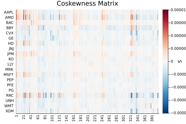
Cokurtosis eigenspectrum: vanilla vs denoised.
plot_coskewness(prs[2].second, rd)
Cokurtosis eigenspectrum: denoised.
plot_cokurtosis(prs[1].second, rd)
plot_cokurtosis(prs[2].second, rd)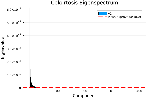
4. Why it matters: skew- and tail-aware optimisation
We minimise two high-order risk measures — NegativeSkewness and Kurtosis — using each high-order prior. With the raw (near-singular) tensors the solver is working against a degenerate problem; the denoised and sparsified priors give stable, sensible allocations.
using Clarabel

slv = Solver(; name = :clarabel1, solver = Clarabel.Optimizer,
             settings = Dict("verbose" => false),
             check_sol = (; allow_local = true, allow_almost = true))

ress_sk = [k => optimise(MeanRisk(; r = NegativeSkewness(), obj = MinimumRisk(),
                                  opt = JuMPOptimiser(; pe = p, slv = slv)))
           for (k, p) in prs]
ress_kt = [k => optimise(MeanRisk(; r = Kurtosis(), obj = MinimumRisk(),
                                  opt = JuMPOptimiser(; pe = p, slv = slv)))
           for (k, p) in prs]

pretty_table(DataFrame(["Assets" => rd.nx;
                        ["NSkew $k" => r.w for (k, r) in ress_sk];
                        ["Kurt $k" => r.w for (k, r) in ress_kt]]); formatters = [resfmt],
             title = "Minimum skew / kurtosis weights by prior")
Minimum skew / kurtosis weights by prior
┌────────┬───────────────┬───────────────┬────────────┬──────────────┬──────────
│ Assets │ NSkew Vanilla │ NSkew Denoise │ NSkew LoGo │ Kurt Vanilla │ Kurt De ⋯
│ String │ Float64 │ Float64 │ Float64 │ Float64 │ Fl ⋯
├────────┼───────────────┼───────────────┼────────────┼──────────────┼──────────
│ AAPL │ 0.0 % │ 2.907 % │ 2.566 % │ 0.0 % │ ⋯
│ AMD │ 0.0 % │ 0.0 % │ 0.0 % │ 0.0 % │ ⋯
│ BAC │ 15.073 % │ 14.784 % │ 24.03 % │ 0.0 % │ ⋯
│ BBY │ 0.0 % │ 0.0 % │ 0.0 % │ 0.0 % │ ⋯
│ CVX │ 5.941 % │ 4.424 % │ 0.474 % │ 0.0 % │ 0. ⋯
│ GE │ 0.0 % │ 0.0 % │ 0.0 % │ 1.548 % │ 1. ⋯
│ HD │ 0.0 % │ 0.0 % │ 0.0 % │ 2.616 % │ 2. ⋯
│ JNJ │ 16.214 % │ 19.119 % │ 12.823 % │ 40.295 % │ 40. ⋯
│ JPM │ 30.097 % │ 31.236 % │ 19.829 % │ 2.471 % │ 2. ⋯
│ KO │ 0.794 % │ 0.0 % │ 0.0 % │ 1.878 % │ 0. ⋯
│ LLY │ 7.921 % │ 4.237 % │ 13.699 % │ 0.0 % │ ⋯
│ MRK │ 14.537 % │ 12.854 % │ 21.285 % │ 25.182 % │ 23. ⋯
│ MSFT │ 7.633 % │ 7.475 % │ 1.05 % │ 0.0 % │ ⋯
│ PEP │ 0.0 % │ 0.0 % │ 0.0 % │ 0.0 % │ 2. ⋯
│ ⋮ │ ⋮ │ ⋮ │ ⋮ │ ⋮ │ ⋱
└────────┴───────────────┴───────────────┴────────────┴──────────────┴──────────
2 columns and 6 rows omittedThe composition plot contrasts the negative skew-minimising portfolios across the three priors.
plot_stacked_bar_composition([r for (_, r) in ress_sk], rd;
                             xticks = (1:length(ress_sk), [k for (k, _) in ress_sk]))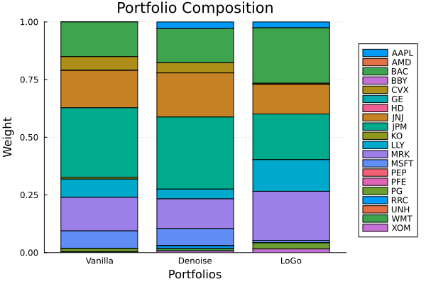
The composition plot contrasts the kurtosis-minimising portfolios across the three priors.
plot_stacked_bar_composition([r for (_, r) in ress_kt], rd;
                             xticks = (1:length(ress_kt), [k for (k, _) in ress_kt]))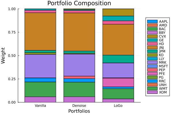
This page was generated using Literate.jl.