
The source files can be found in examples/.
Clustering optimisers with mixed risks and constraints
This example turns the clustering optimiser chapter into a deeper playground for two things that are easy to miss in the overview:
clustering optimisers can mix risk measures and scalarisers across the hierarchy;
the hierarchical optimiser can still carry constraints and fees while the cluster logic does the diversification work.
We use the same S&P 500 slice as the rest of the examples, then compare a plain HRP solve, several mixed-risk HERC variants, and a constrained HERC solve.
When to reach for this
Reach for mixed-risk clustering optimisers when no single risk measure captures what you care about and you still want the hierarchy to do the diversification — for example combining a tail measure with variance, or treating intra-cluster and inter-cluster risk differently. The clustering structure keeps the allocation robust while the scalariser controls how the mixed risk terms combine.
using PortfolioOptimisers, PrettyTables

resfmt = (v, i, j) -> begin
    if j == 1
        return v
    else
        return isa(v, Number) ? "$(round(v * 100, digits = 3)) %" : v
    end
end;
1. Data and clustering
We compute the prior and cluster hierarchy once, then reuse them across all the examples.
using CSV, TimeSeries, DataFrames, Clarabel

X = TimeArray(CSV.File(joinpath(@__DIR__, "..", "SP500.csv.gz")); timestamp = :Date)[(end - 252):end]
rd = prices_to_returns(X)
pr = prior(EmpiricalPrior(), rd)
clr = clusterise(ClustersEstimator(; alg = DBHT()), pr.X)

# Shared solver and hierarchical optimiser.
slv = Solver(; name = :clarabel, solver = Clarabel.Optimizer,
             settings = Dict("verbose" => false),
             check_sol = (; allow_local = true, allow_almost = true))
opt = HierarchicalOptimiser(; pe = pr, cle = clr, slv = slv)
HierarchicalOptimiser
pe ┼ LowOrderPrior
│ X ┼ 252×20 Matrix{Float64}
│ mu ┼ 20-element Vector{Float64}
│ sigma ┼ 20×20 Matrix{Float64}
│ chol ┼ nothing
│ w ┼ nothing
│ ens ┼ nothing
│ kld ┼ nothing
│ ow ┼ nothing
│ rr ┼ nothing
│ f_mu ┼ nothing
│ f_sigma ┼ nothing
│ f_w ┴ nothing
cle ┼ Clusters
│ res ┼ Clustering.Hclust{Float64}([-1 -13; -7 -4; … ; 12 17; 10 18], [0.1, 0.1111111111111111, 0.125, 0.14285714285714285, 0.16666666666666666, 0.2, 0.25, 0.3333333333333333, 0.5, 1.0, 0.125, 0.14285714285714285, 0.16666666666666666, 0.2, 0.25, 0.3333333333333333, 0.5, 1.0, 2.0], [5, 20, 17, 3, 9, 6, 2, 1, 13, 7, 4, 19, 14, 10, 16, 18, 11, 8, 12, 15], :DBHT)
│ S ┼ 20×20 Matrix{Float64}
│ D ┼ 20×20 Matrix{Float64}
│ P ┼ nothing
│ k ┴ Int64: 4
slv ┼ Solver
│ name ┼ Symbol: :clarabel
│ solver ┼ UnionAll: Clarabel.MOIwrapper.Optimizer
│ settings ┼ Dict{String, Bool}: Dict{String, Bool}("verbose" => 0)
│ check_sol ┼ @NamedTuple{allow_local::Bool, allow_almost::Bool}: (allow_local = true, allow_almost = true)
│ add_bridges ┴ Bool: true
wb ┼ WeightBounds
│ lb ┼ Float64: 0.0
│ ub ┴ Float64: 1.0
fees ┼ nothing
sets ┼ nothing
wf ┼ IterativeWeightFinaliser
│ iter ┴ Int64: 100
brt ┼ Bool: false
cle_pr ┼ Bool: true
strict ┴ Bool: false2. HRP with mixed risk measures
HierarchicalRiskParity accepts either a single risk measure or a vector of them. When we pass a vector, the scalariser chooses how to combine the inner risk terms.
Here we mix tail risk and variance, then sweep a few scalarisers to show that the hierarchy really is responding to the combination rule rather than to a single hidden default.
r_mix = [ConditionalValueatRisk(),
         Variance(; settings = RiskMeasureSettings(; scale = 2e2))]
hrp_sum = optimise(HierarchicalRiskParity(; r = r_mix, opt = opt, sca = SumScalariser()))
hrp_max = optimise(HierarchicalRiskParity(; r = r_mix, opt = opt, sca = MaxScalariser()))
hrp_min = optimise(HierarchicalRiskParity(; r = r_mix, opt = opt, sca = MinScalariser()))
hrp_lse = optimise(HierarchicalRiskParity(; r = r_mix, opt = opt,
                                          sca = LogSumExpScalariser(; gamma = 1e2)))

pretty_table(DataFrame(; :assets => rd.nx, :Sum => hrp_sum.w, :Max => hrp_max.w,
                       :Min => hrp_min.w, :LogSumExp => hrp_lse.w); formatters = [resfmt])
┌────────┬──────────┬──────────┬──────────┬───────────┐
│ assets │ Sum │ Max │ Min │ LogSumExp │
│ String │ Float64 │ Float64 │ Float64 │ Float64 │
├────────┼──────────┼──────────┼──────────┼───────────┤
│ AAPL │ 3.866 % │ 3.26 % │ 4.801 % │ 3.937 % │
│ AMD │ 1.669 % │ 1.263 % │ 2.678 % │ 1.53 % │
│ BAC │ 3.785 % │ 3.356 % │ 4.017 % │ 4.005 % │
│ BBY │ 3.373 % │ 2.871 % │ 4.403 % │ 3.0 % │
│ CVX │ 4.403 % │ 3.937 % │ 4.891 % │ 4.7 % │
│ GE │ 4.208 % │ 3.879 % │ 4.133 % │ 4.691 % │
│ HD │ 2.751 % │ 2.605 % │ 2.72 % │ 3.118 % │
│ JNJ │ 11.741 % │ 13.136 % │ 10.025 % │ 10.95 % │
│ JPM │ 4.293 % │ 3.965 % │ 4.208 % │ 4.713 % │
│ KO │ 5.384 % │ 6.299 % │ 4.426 % │ 5.189 % │
│ LLY │ 6.556 % │ 5.995 % │ 7.372 % │ 6.223 % │
│ MRK │ 6.076 % │ 6.583 % │ 5.297 % │ 5.813 % │
│ MSFT │ 2.345 % │ 2.06 % │ 2.675 % │ 2.477 % │
│ PEP │ 9.848 % │ 11.24 % │ 8.327 % │ 9.598 % │
│ PFE │ 3.77 % │ 3.589 % │ 3.965 % │ 3.553 % │
│ ⋮ │ ⋮ │ ⋮ │ ⋮ │ ⋮ │
└────────┴──────────┴──────────┴──────────┴───────────┘
5 rows omitted3. HERC with mixed inner and outer risks
HierarchicalEqualRiskContribution lets the inner and outer levels use different risk measures and scalarisers. That makes it the cleanest place to show the "mixed risk" idea: the hierarchy can treat intra-cluster and inter-cluster risk differently.
We pair the same mixed risk vector at both levels, then vary the scalariser to show the contrast between additive, max, min, and log-sum-exp aggregation.
herc_sum = optimise(HierarchicalEqualRiskContribution(; opt = opt, ri = r_mix, ro = r_mix,
                                                      scai = SumScalariser(),
                                                      scao = SumScalariser()))
herc_max = optimise(HierarchicalEqualRiskContribution(; opt = opt, ri = r_mix, ro = r_mix,
                                                      scai = MaxScalariser(),
                                                      scao = MaxScalariser()))
herc_min = optimise(HierarchicalEqualRiskContribution(; opt = opt, ri = r_mix, ro = r_mix,
                                                      scai = MinScalariser(),
                                                      scao = MinScalariser()))
herc_lse = optimise(HierarchicalEqualRiskContribution(; opt = opt, ri = r_mix, ro = r_mix,
                                                      scai = LogSumExpScalariser(;
                                                                                 gamma = 1e2),
                                                      scao = LogSumExpScalariser(;
                                                                                 gamma = 1e2)))

pretty_table(DataFrame(; :assets => rd.nx, :Sum => herc_sum.w, :Max => herc_max.w,
                       :Min => herc_min.w, :LogSumExp => herc_lse.w); formatters = [resfmt])
┌────────┬──────────┬──────────┬──────────┬───────────┐
│ assets │ Sum │ Max │ Min │ LogSumExp │
│ String │ Float64 │ Float64 │ Float64 │ Float64 │
├────────┼──────────┼──────────┼──────────┼───────────┤
│ AAPL │ 2.124 % │ 1.857 % │ 2.628 % │ 2.175 % │
│ AMD │ 0.723 % │ 0.63 % │ 1.445 % │ 0.738 % │
│ BAC │ 2.552 % │ 2.232 % │ 2.998 % │ 2.614 % │
│ BBY │ 1.31 % │ 1.144 % │ 1.969 % │ 1.34 % │
│ CVX │ 5.519 % │ 4.547 % │ 6.078 % │ 5.41 % │
│ GE │ 2.21 % │ 1.934 % │ 2.23 % │ 2.266 % │
│ HD │ 2.739 % │ 2.398 % │ 2.629 % │ 2.809 % │
│ JNJ │ 10.319 % │ 10.791 % │ 7.863 % │ 10.128 % │
│ JPM │ 3.013 % │ 2.636 % │ 3.141 % │ 3.088 % │
│ KO │ 12.774 % │ 13.746 % │ 10.942 % │ 13.001 % │
│ LLY │ 4.226 % │ 4.407 % │ 5.503 % │ 4.136 % │
│ MRK │ 7.883 % │ 8.24 % │ 6.658 % │ 7.733 % │
│ MSFT │ 2.168 % │ 1.896 % │ 2.586 % │ 2.221 % │
│ PEP │ 13.062 % │ 14.058 % │ 10.897 % │ 13.296 % │
│ PFE │ 4.304 % │ 4.492 % │ 4.984 % │ 4.216 % │
│ ⋮ │ ⋮ │ ⋮ │ ⋮ │ ⋮ │
└────────┴──────────┴──────────┴──────────┴───────────┘
5 rows omittedThe scalariser choice can dominate the solution when one risk measure is consistently larger than the other. That is why the max and min solutions can collapse toward the portfolio that is effectively minimising the dominating term.
using StatsPlots, GraphRecipes
plot_stacked_bar_composition([hrp_sum, hrp_max, hrp_min, hrp_lse, herc_sum, herc_max,
                              herc_min, herc_lse], rd)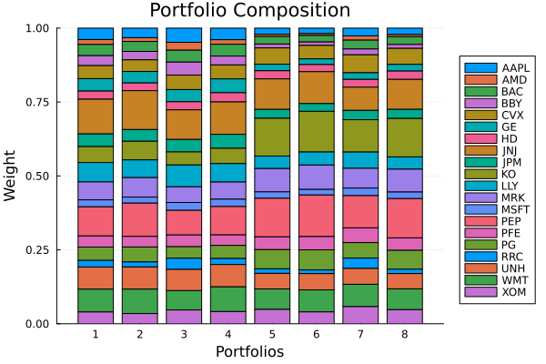
4. Constrained HERC
The hierarchical optimiser itself can still carry weight bounds and fees. This version keeps the same mixed risk structure, but asks the optimiser to stay inside a bounded, fee-aware universe. We set a 10% cap (ub = 0.1) deliberately tight enough to bind: the unconstrained HERC already concentrates around 13% in the largest names, so the cap pulls them down — watch the largest holdings in the comparison below.
opt_constrained = HierarchicalOptimiser(; pe = pr, cle = clr, slv = slv,
                                        wb = WeightBounds(; lb = 0.0, ub = 0.1),
                                        fees = Fees(; l = 0.001))
herc_constrained = optimise(HierarchicalEqualRiskContribution(; opt = opt_constrained,
                                                              ri = r_mix, ro = r_mix,
                                                              scai = SumScalariser(),
                                                              scao = SumScalariser()))

pretty_table(DataFrame(; :assets => rd.nx, :Unconstrained => herc_sum.w,
                       :Constrained => herc_constrained.w); formatters = [resfmt])
┌────────┬───────────────┬─────────────┐
│ assets │ Unconstrained │ Constrained │
│ String │ Float64 │ Float64 │
├────────┼───────────────┼─────────────┤
│ AAPL │ 2.124 % │ 2.342 % │
│ AMD │ 0.723 % │ 0.797 % │
│ BAC │ 2.552 % │ 2.814 % │
│ BBY │ 1.31 % │ 1.444 % │
│ CVX │ 5.519 % │ 6.105 % │
│ GE │ 2.21 % │ 2.437 % │
│ HD │ 2.739 % │ 3.021 % │
│ JNJ │ 10.319 % │ 10.0 % │
│ JPM │ 3.013 % │ 3.322 % │
│ KO │ 12.774 % │ 10.0 % │
│ LLY │ 4.226 % │ 4.604 % │
│ MRK │ 7.883 % │ 8.586 % │
│ MSFT │ 2.168 % │ 2.391 % │
│ PEP │ 13.062 % │ 10.0 % │
│ PFE │ 4.304 % │ 4.689 % │
│ ⋮ │ ⋮ │ ⋮ │
└────────┴───────────────┴─────────────┘
5 rows omittedThe risk-contribution view shows how the hierarchy spreads risk rather than capital. Populate the covariance via factory before calling plot_risk_contribution.
rv = factory(Variance(), pr)
plot_risk_contribution(rv, herc_constrained, rd)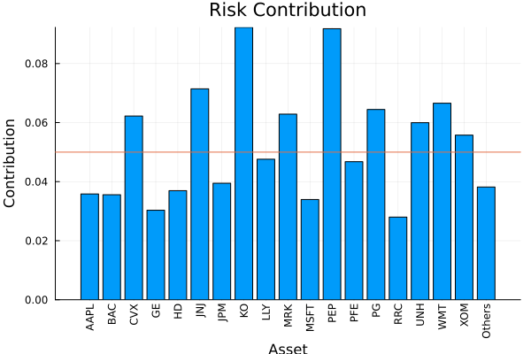
Summary
Clustering optimisers give you a hierarchical lever on diversification.
HierarchicalRiskParityresponds to the scalariser when you mix risk measures.HierarchicalEqualRiskContributionlets inner and outer levels use different risk terms and different scalarisers.HierarchicalOptimisercan still carry practical constraints like weight bounds and fees while the hierarchy does the allocation.
This page was generated using Literate.jl.