
The source files can be found in examples/.
Nested clustered optimisation with layered constraints and fees
This example shows how to apply constraints at three distinct layers of NestedClustered:
the inner optimisation within each cluster,
the outer optimisation across synthetic cluster portfolios,
and a final overall optimisation pass on the full universe.
It also shows how fees can be attached to the nested stage and to the final overall stage.
When to reach for this
Reach for this when you want cluster structure for robustness, but still need practical controls (fees and weight limits) at more than one stage of the nested workflow.
using PortfolioOptimisers, PrettyTables, StableRNGs

resfmt = (v, i, j) -> begin
    if j == 1
        return v
    else
        return isa(v, Number) ? "$(round(v * 100, digits = 3)) %" : v
    end
end;
1. Data and shared setup
We use one year of S&P 500 data and compute clusters once. Then we compare three nested setups:
inner-only weight bounds,
inner + outer bounds plus fees in the nested stage,
direct overall asset bounds on
NestedClustered.
using CSV, TimeSeries, DataFrames, Clarabel

X = TimeArray(CSV.File(joinpath(@__DIR__, "..", "SP500.csv.gz")); timestamp = :Date)[(end - 252):end]
rd = prices_to_returns(X)

slv = [Solver(; name = :clarabel1, solver = Clarabel.Optimizer,
              settings = Dict("verbose" => false),
              check_sol = (; allow_local = true, allow_almost = true)),
       Solver(; name = :clarabel2, solver = Clarabel.Optimizer,
              settings = Dict("verbose" => false, "max_step_fraction" => 0.95),
              check_sol = (; allow_local = true, allow_almost = true)),
       Solver(; name = :clarabel3, solver = Clarabel.Optimizer,
              settings = Dict("verbose" => false, "max_step_fraction" => 0.9),
              check_sol = (; allow_local = true, allow_almost = true))]

pr = prior(EmpiricalPrior(), rd)
clr = clusterise(ClustersEstimator(; alg = DBHT()), pr.X)
Clusters
res ┼ Clustering.Hclust{Float64}([-1 -13; -7 -4; … ; 12 17; 10 18], [0.1, 0.1111111111111111, 0.125, 0.14285714285714285, 0.16666666666666666, 0.2, 0.25, 0.3333333333333333, 0.5, 1.0, 0.125, 0.14285714285714285, 0.16666666666666666, 0.2, 0.25, 0.3333333333333333, 0.5, 1.0, 2.0], [5, 20, 17, 3, 9, 6, 2, 1, 13, 7, 4, 19, 14, 10, 16, 18, 11, 8, 12, 15], :DBHT)
S ┼ 20×20 Matrix{Float64}
D ┼ 20×20 Matrix{Float64}
P ┼ nothing
k ┴ Int64: 42. Layering constraints in NCO
The nested workflow solves:
The key wiring rule remains the same: the outer optimiser must not consume the asset-level prior directly; it works on synthetic cluster returns.
jopti_inner = JuMPOptimiser(; pe = pr, slv = slv, wb = WeightBounds(; lb = 0.0, ub = 0.35))
jopto_base = JuMPOptimiser(; slv = slv)
jopto_outer = JuMPOptimiser(; slv = slv, wb = WeightBounds(; lb = 0.0, ub = 0.62))

res_inner = optimise(NestedClustered(; pe = pr, cle = clr,
                                     opti = MeanRisk(; obj = MinimumRisk(),
                                                     opt = jopti_inner),
                                     opto = MeanRisk(; obj = MinimumRisk(),
                                                     opt = jopto_base)), rd)

res_inner_outer = optimise(NestedClustered(; pe = pr, cle = clr, fees = Fees(; l = 0.001),
                                           opti = MeanRisk(; obj = MinimumRisk(),
                                                           opt = jopti_inner),
                                           opto = MeanRisk(; obj = MinimumRisk(),
                                                           opt = jopto_outer)), rd)

wb_overall_assets = WeightBounds(; lb = fill(0.0, length(rd.nx)),
                                 ub = fill(0.20, length(rd.nx)))
WeightBounds
lb ┼ 20-element Vector{Float64}
ub ┴ 20-element Vector{Float64}Use per-asset vectors so the direct NestedClustered(wb = ...) bound is applied to final aggregated asset weights (not just cluster allocations).
res_nested_overall = optimise(NestedClustered(; pe = pr, cle = clr, wb = wb_overall_assets,
                                              fees = Fees(; l = 0.001),
                                              opti = MeanRisk(; obj = MinimumRisk(),
                                                              opt = jopti_inner),
                                              opto = MeanRisk(; obj = MinimumRisk(),
                                                              opt = jopto_outer)), rd)

pretty_table(DataFrame(; :assets => rd.nx, :InnerOnlyWB => res_inner.w,
                       :InnerOuterWBFees => res_inner_outer.w,
                       :NestedDirectOverallWB => res_nested_overall.w);
             formatters = [resfmt])
┌────────┬─────────────┬──────────────────┬───────────────────────┐
│ assets │ InnerOnlyWB │ InnerOuterWBFees │ NestedDirectOverallWB │
│ String │ Float64 │ Float64 │ Float64 │
├────────┼─────────────┼──────────────────┼───────────────────────┤
│ AAPL │ 0.0 % │ 0.0 % │ 0.0 % │
│ AMD │ 0.0 % │ 0.0 % │ 0.0 % │
│ BAC │ 0.0 % │ 0.0 % │ 0.0 % │
│ BBY │ 0.0 % │ 0.0 % │ 0.0 % │
│ CVX │ 3.274 % │ 3.304 % │ 3.458 % │
│ GE │ 0.0 % │ 0.0 % │ 0.0 % │
│ HD │ 0.0 % │ 0.0 % │ 0.0 % │
│ JNJ │ 22.366 % │ 21.7 % │ 20.0 % │
│ JPM │ 0.0 % │ 0.0 % │ 0.0 % │
│ KO │ 9.36 % │ 9.996 % │ 10.463 % │
│ LLY │ 0.0 % │ 0.0 % │ 0.0 % │
│ MRK │ 21.618 % │ 20.975 % │ 20.0 % │
│ MSFT │ 0.0 % │ 0.0 % │ 0.0 % │
│ PEP │ 9.36 % │ 9.996 % │ 10.463 % │
│ PFE │ 0.264 % │ 0.256 % │ 0.268 % │
│ ⋮ │ ⋮ │ ⋮ │ ⋮ │
└────────┴─────────────┴──────────────────┴───────────────────────┘
5 rows omittedThe following audit confirms where the constraints are active.
Inner bound (
0.35) applies to each cluster-level solve.Outer bound (
0.62) applies to cluster allocation weights.Overall bound (
0.20) can be applied directly inNestedClustered, applied here using per-asset vector bounds.
inner_local_max(res) = maximum(maximum(ri.w) for ri in res.resi)
outer_cluster_max(res) = maximum(res.reso.w)

audit = DataFrame(:Metric => ["Max inner local weight", "Max outer cluster weight",
                              "Max final asset weight"], :Limit => [0.35, 0.62, 0.20],
                  :NestedInnerOnly =>
                      [inner_local_max(res_inner), maximum(res_inner.reso.w),
                       maximum(res_inner.w)],
                  :NestedInnerOuterFees =>
                      [inner_local_max(res_inner_outer), outer_cluster_max(res_inner_outer),
                       maximum(res_inner_outer.w)],
                  :NestedDirectOverallWB => [inner_local_max(res_nested_overall),
                                             outer_cluster_max(res_nested_overall),
                                             maximum(res_nested_overall.w)])

pretty_table(audit; formatters = [resfmt])
┌──────────────────────────┬─────────┬─────────────────┬────────────────────────
│ Metric │ Limit │ NestedInnerOnly │ NestedInnerOuterFees ⋯
│ String │ Float64 │ Float64 │ Float64 ⋯
├──────────────────────────┼─────────┼─────────────────┼────────────────────────
│ Max inner local weight │ 35.0 % │ 35.0 % │ 35.0 % ⋯
│ Max outer cluster weight │ 62.0 % │ 63.903 % │ 62.0 % ⋯
│ Max final asset weight │ 20.0 % │ 22.366 % │ 21.7 % ⋯
└──────────────────────────┴─────────┴─────────────────┴────────────────────────
1 column omittedThese runs isolate layer placement:
inner bounds shape per-cluster compositions,
outer bounds shape allocation across clusters,
direct
NestedClustered(wb = ...)bounds constrain the final aggregated asset weights.
using StatsPlots, GraphRecipes
plot_stacked_bar_composition([res_inner, res_inner_outer, res_nested_overall], rd;
                             xticks = ([1, 2, 3],
                                       ["Inner WB", "Inner+Outer WB+Fees", "Overall WB"]))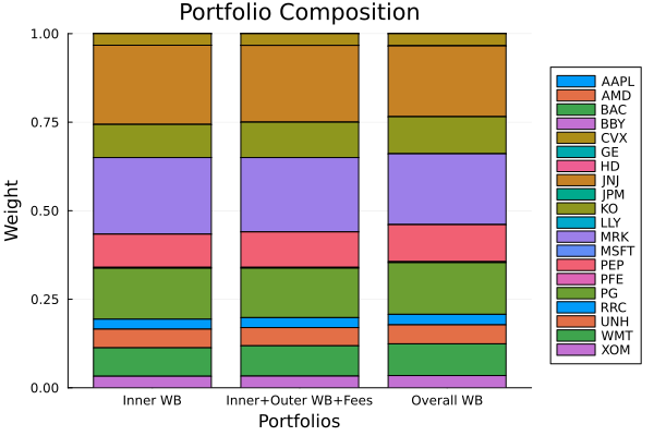
Summary
Layered controls can be applied around NestedClustered without giving up the cluster-based decomposition.
Inner
wbcontrols weights inside each cluster.Outer
wbcontrols allocation across synthetic cluster portfolios.Direct
NestedClustered(wb = ...)can constrain final asset weights when provided with a weight bounds result or estimator.
This page was generated using Literate.jl.