
The source files can be found in examples/.
Entropy pooling
Black–Litterman blends views into the mean through a Gaussian update. Entropy pooling is more general in two ways. First, it expresses views as constraints on any moment — mean, variance, CVaR, skewness, kurtosis, even individual covariances and correlations. Second, it does not assume normality: it reweights the empirical scenarios so that the new distribution satisfies your views while staying as close as possible (in relative entropy / Kullback–Leibler divergence) to the original. The output is a fully reweighted prior, not just a shifted mean.
This is the second page of the view-prior arc — Black–Litterman came first, and Opinion Pooling follows, combining several entropy-pooling views into one.
In PortfolioOptimisers, EntropyPoolingPrior accepts a separate LinearConstraintEstimator per quantity. Mind the naming: mu_views is the mean, sigma_views is the variance, var_views is the Value at Risk and cvar_views the Conditional VaR (tail-risk views), sk_views/kt_views are skewness/kurtosis, and cov_views/rho_views target covariances/correlations. Each is a list of string constraints over the AssetSets names.
When to reach for this
Reach for entropy pooling when your views are richer than "the mean will be x": views on volatility, tail risk (CVaR), skewness, or the correlation between two assets, possibly several at once. It is also the right tool when you distrust the normality assumption baked into Black–Litterman, since it reweights the empirical scenarios directly. For a simple mean-only view, Black–Litterman is lighter; to combine several entropy-pooling opinions, see Opinion Pooling.
using PortfolioOptimisers, PrettyTables

mmtfmt = (v, i, j) -> begin
    if j == 1
        return v
    else
        return isa(v, Number) ? "$(round(v*100, digits=4)) %" : v
    end
end;
resfmt = (v, i, j) -> begin
    if j == 1
        return v
    else
        return isa(v, Number) ? "$(round(v*100, digits=3)) %" : v
    end
end;
1. ReturnsResult data
We use the same S&P 500 slice as the other examples.
using CSV, TimeSeries, DataFrames

X = TimeArray(CSV.File(joinpath(@__DIR__, "..", "SP500.csv.gz")); timestamp = :Date)[(end - 252):end]
rd = prices_to_returns(X)
ReturnsResult
nx ┼ 20-element Vector{String}
X ┼ 252×20 Matrix{Float64}
nf ┼ nothing
F ┼ nothing
nb ┼ nothing
B ┼ nothing
ts ┼ 252-element Vector{Date}
iv ┼ nothing
ivpa ┴ nothing2. Naming assets and groups
As with Black–Litterman, views reference assets and groups by name through an AssetSets.
sets = AssetSets(;
                 dict = Dict("nx" => rd.nx, "tech" => ["AAPL", "AMD", "MSFT"],
                             "energy" => ["CVX"]))
AssetSets
key ┼ String: "nx"
ukey ┼ String: "ux"
dict ┴ Dict{String, Vector{String}}: Dict("nx" => ["AAPL", "AMD", "BAC", "BBY", "CVX", "GE", "HD", "JNJ", "JPM", "KO", "LLY", "MRK", "MSFT", "PEP", "PFE", "PG", "RRC", "UNH", "WMT", "XOM"], "tech" => ["AAPL", "AMD", "MSFT"], "energy" => ["CVX"])3. Views on several moments
Entropy-pooling views are also plain strings, but they can target different quantities. Here we state a mean view (Apple returns 8 bps) via mu_views, a relative mean view (tech outperforms energy), and a variance view (pin Apple's variance) via sigma_views. The comparison operators a view accepts depend on the moment: mu_views, sigma_views, sk_views, kt_views, cov_views and rho_views take ==, >= and <=; var_views (VaR) takes only == and >=; and cvar_views (CVaR) takes only ==. An unsupported operator raises a ParseError listing the ones allowed for that view.
mu_views = LinearConstraintEstimator(; val = ["AAPL == 0.0008", "tech >= energy"])
sigma_views = LinearConstraintEstimator(; val = ["AAPL == 0.0003"])

ep = EntropyPoolingPrior(; sets = sets, mu_views = mu_views, sigma_views = sigma_views)
EntropyPoolingPrior
pe ┼ EmpiricalPrior
│ ce ┼ PortfolioOptimisersCovariance
│ │ ce ┼ Covariance
│ │ │ me ┼ SimpleExpectedReturns
│ │ │ │ w ┴ nothing
│ │ │ ce ┼ GeneralCovariance
│ │ │ │ ce ┼ SimpleCovariance: SimpleCovariance(true)
│ │ │ │ w ┴ nothing
│ │ │ alg ┴ FullMoment()
│ │ mp ┼ MatrixProcessing
│ │ │ pdm ┼ Posdef
│ │ │ │ alg ┼ UnionAll: NearestCorrelationMatrix.Newton
│ │ │ │ kwargs ┴ @NamedTuple{}: NamedTuple()
│ │ │ dn ┼ nothing
│ │ │ dt ┼ nothing
│ │ │ alg ┼ nothing
│ │ │ order ┴ NTuple{4, Symbol}: (:pdm, :dn, :dt, :alg)
│ me ┼ SimpleExpectedReturns
│ │ w ┴ nothing
│ horizon ┴ nothing
mu_views ┼ LinearConstraintEstimator
│ val ┼ Vector{String}: ["AAPL == 0.0008", "tech >= energy"]
│ key ┴ nothing
var_views ┼ nothing
cvar_views ┼ nothing
sigma_views ┼ LinearConstraintEstimator
│ val ┼ Vector{String}: ["AAPL == 0.0003"]
│ key ┴ nothing
sk_views ┼ nothing
kt_views ┼ nothing
cov_views ┼ nothing
rho_views ┼ nothing
var_alpha ┼ nothing
cvar_alpha ┼ nothing
sets ┼ AssetSets
│ key ┼ String: "nx"
│ ukey ┼ String: "ux"
│ dict ┴ Dict{String, Vector{String}}: Dict("nx" => ["AAPL", "AMD", "BAC", "BBY", "CVX", "GE", "HD", "JNJ", "JPM", "KO", "LLY", "MRK", "MSFT", "PEP", "PFE", "PG", "RRC", "UNH", "WMT", "XOM"], "tech" => ["AAPL", "AMD", "MSFT"], "energy" => ["CVX"])
ds_opt ┼ nothing
dm_opt ┼ nothing
opt ┼ OptimEntropyPooling
│ args ┼ Tuple{}: ()
│ kwargs ┼ @NamedTuple{}: NamedTuple()
│ sc1 ┼ Int64: 1
│ sc2 ┼ Float64: 1000.0
│ alg ┼ ExpEntropyPooling()
│ err ┴ nothing
w ┼ nothing
alg ┴ H1_EntropyPooling()4. Prior vs reweighted posterior
We compute the entropy-pooling posterior and compare both the mean and the variance of Apple against the plain empirical prior — the mean view lifts the expected return while the variance view tightens the dispersion, exactly as instructed.
pr_ep = prior(ep, rd)
pr_emp = prior(EmpiricalPrior(), rd)

i_aapl = findfirst(==("AAPL"), rd.nx)
pretty_table(DataFrame(["moment" => ["mean (AAPL)", "variance (AAPL)"],
                        "Empirical" => [pr_emp.mu[i_aapl], pr_emp.sigma[i_aapl, i_aapl]],
                        "Entropy pooling" =>
                            [pr_ep.mu[i_aapl], pr_ep.sigma[i_aapl, i_aapl]]]);
             formatters = [mmtfmt],
             title = "Apple moments: empirical vs entropy-pooling view")
Apple moments: empirical vs entropy-pooling view
┌─────────────────┬───────────┬─────────────────┐
│ moment │ Empirical │ Entropy pooling │
│ String │ Float64 │ Float64 │
├─────────────────┼───────────┼─────────────────┤
│ mean (AAPL) │ -0.1126 % │ 0.08 % │
│ variance (AAPL) │ 0.05 % │ 0.0301 % │
└─────────────────┴───────────┴─────────────────┘The full expected-returns vectors, side by side.
pretty_table(DataFrame(["Assets" => rd.nx, "Empirical" => pr_emp.mu,
                        "Entropy pooling" => pr_ep.mu]); formatters = [mmtfmt],
             title = "Expected returns: empirical vs entropy-pooling posterior")
Expected returns: empirical vs entropy-pooling posterior
┌────────┬───────────┬─────────────────┐
│ Assets │ Empirical │ Entropy pooling │
│ String │ Float64 │ Float64 │
├────────┼───────────┼─────────────────┤
│ AAPL │ -0.1126 % │ 0.08 % │
│ AMD │ -0.2809 % │ 0.0698 % │
│ BAC │ -0.0934 % │ -0.0124 % │
│ BBY │ -0.0279 % │ 0.1921 % │
│ CVX │ 0.1945 % │ 0.243 % │
│ GE │ -0.0339 % │ 0.1278 % │
│ HD │ -0.0707 % │ 0.0504 % │
│ JNJ │ 0.0307 % │ 0.0766 % │
│ JPM │ -0.0417 % │ 0.0256 % │
│ KO │ 0.0497 % │ 0.098 % │
│ LLY │ 0.1305 % │ 0.1942 % │
│ MRK │ 0.1669 % │ 0.1861 % │
│ MSFT │ -0.1206 % │ 0.0932 % │
│ PEP │ 0.039 % │ 0.1159 % │
│ ⋮ │ ⋮ │ ⋮ │
└────────┴───────────┴─────────────────┘
6 rows omittedEntropy-pooling posterior expected returns.
using StatsPlots, GraphRecipes
plot_mu(pr_ep, rd.nx)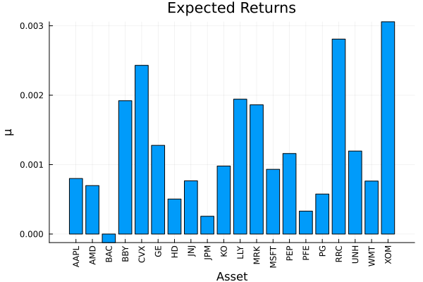
5. Why it matters: views change the portfolio
Feeding the reweighted prior to a return-seeking optimiser tilts the portfolio toward the view-favoured assets, just as Black–Litterman did — but here the whole distribution, not only the mean, has been updated.
using Clarabel

slv = Solver(; name = :clarabel1, solver = Clarabel.Optimizer,
             settings = Dict("verbose" => false),
             check_sol = (; allow_local = true, allow_almost = true))
rf = 4.2 / 100 / 252

res_emp = optimise(MeanRisk(; obj = MaximumRatio(; rf = rf),
                            opt = JuMPOptimiser(; pe = pr_emp, slv = slv)))
res_ep = optimise(MeanRisk(; obj = MaximumRatio(; rf = rf),
                           opt = JuMPOptimiser(; pe = pr_ep, slv = slv)))

pretty_table(DataFrame(["Assets" => rd.nx, "Empirical" => res_emp.w,
                        "Entropy pooling" => res_ep.w]); formatters = [resfmt],
             title = "Maximum-ratio weights: empirical vs entropy pooling")
Maximum-ratio weights: empirical vs entropy pooling
┌────────┬───────────┬─────────────────┐
│ Assets │ Empirical │ Entropy pooling │
│ String │ Float64 │ Float64 │
├────────┼───────────┼─────────────────┤
│ AAPL │ 0.0 % │ 0.0 % │
│ AMD │ 0.0 % │ 0.0 % │
│ BAC │ 0.0 % │ 0.0 % │
│ BBY │ 0.0 % │ 6.52 % │
│ CVX │ 0.0 % │ 0.0 % │
│ GE │ 0.0 % │ 0.0 % │
│ HD │ 0.0 % │ 0.0 % │
│ JNJ │ 0.0 % │ 0.0 % │
│ JPM │ 0.0 % │ 0.0 % │
│ KO │ 0.0 % │ 0.0 % │
│ LLY │ 0.002 % │ 6.913 % │
│ MRK │ 65.977 % │ 44.433 % │
│ MSFT │ 0.0 % │ 0.0 % │
│ PEP │ 0.0 % │ 12.545 % │
│ ⋮ │ ⋮ │ ⋮ │
└────────┴───────────┴─────────────────┘
6 rows omittedThe composition plot makes the tilt visible.
plot_stacked_bar_composition([res_emp, res_ep], rd;
                             xticks = (1:2, ["Empirical", "Entropy pooling"]))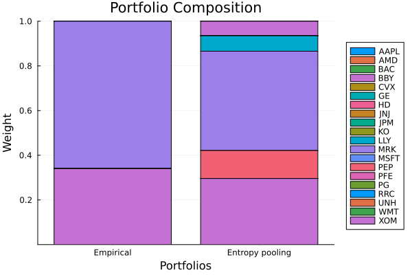
This page was generated using Literate.jl.