
The source files can be found in examples/.
Risk budgeting
RiskBudgeting takes a different stance from MeanRisk. Instead of trading expected return against risk through an objective function, it allocates risk itself: it finds the portfolio whose per-asset (or per-factor) risk contributions match a user-supplied budget as closely as possible. There is no objective to maximise — the budget is the goal.
The classic special case is the equal risk contribution (ERC) portfolio, where every asset contributes the same share of total risk. Risk budgeting generalises it to any budget vector, and to risk measured by any of the risk measures MeanRisk supports.
When to reach for this
Reach for risk budgeting when you care about how risk is distributed rather than about a return/risk trade-off — diversifying risk rather than capital, avoiding the concentration that minimum-variance portfolios are prone to, or expressing a conviction as "this sleeve should carry 30% of the risk". If you instead want the best return for a given risk budget, use MeanRisk.
using PortfolioOptimisers, PrettyTables
# Format for pretty tables.
resfmt = (v, i, j) -> begin
    if j == 1
        return v
    else
        return isa(v, Number) ? "$(round(v*100, digits=3)) %" : v
    end
end;
1. ReturnsResult data
We use one year of S&P 500 constituents, and (for the factor section) the factor returns.
using CSV, TimeSeries, DataFrames

X = TimeArray(CSV.File(joinpath(@__DIR__, "..", "SP500.csv.gz")); timestamp = :Date)[(end - 252):end]
rd = prices_to_returns(X)
ReturnsResult
nx ┼ 20-element Vector{String}
X ┼ 252×20 Matrix{Float64}
nf ┼ nothing
F ┼ nothing
nb ┼ nothing
B ┼ nothing
ts ┼ 252-element Vector{Date}
iv ┼ nothing
ivpa ┴ nothingSince every optimisation below shares the same data, we precompute the prior statistics once with EmpiricalPrior and reuse them, rather than recomputing them on every call.
using Clarabel
slv = Solver(; name = :clarabel, solver = Clarabel.Optimizer,
             settings = Dict("verbose" => false),
             check_sol = (; allow_local = true, allow_almost = true))
pr = prior(EmpiricalPrior(), rd)
opt = JuMPOptimiser(; pe = pr, slv = slv)
JuMPOptimiser
pe ┼ LowOrderPrior
│ X ┼ 252×20 Matrix{Float64}
│ mu ┼ 20-element Vector{Float64}
│ sigma ┼ 20×20 Matrix{Float64}
│ chol ┼ nothing
│ w ┼ nothing
│ ens ┼ nothing
│ kld ┼ nothing
│ ow ┼ nothing
│ rr ┼ nothing
│ f_mu ┼ nothing
│ f_sigma ┼ nothing
│ f_w ┴ nothing
slv ┼ Solver
│ name ┼ Symbol: :clarabel
│ solver ┼ UnionAll: Clarabel.MOIwrapper.Optimizer
│ settings ┼ Dict{String, Bool}: Dict{String, Bool}("verbose" => 0)
│ check_sol ┼ @NamedTuple{allow_local::Bool, allow_almost::Bool}: (allow_local = true, allow_almost = true)
│ add_bridges ┴ Bool: true
wb ┼ WeightBounds
│ lb ┼ Float64: 0.0
│ ub ┴ Float64: 1.0
bgt ┼ Float64: 1.0
sbgt ┼ nothing
lt ┼ nothing
st ┼ nothing
lcse ┼ nothing
cte ┼ nothing
gcarde ┼ nothing
sgcarde ┼ nothing
smtx ┼ nothing
sgmtx ┼ nothing
slt ┼ nothing
sst ┼ nothing
sglt ┼ nothing
sgst ┼ nothing
tn ┼ nothing
fees ┼ nothing
sets ┼ nothing
tr ┼ nothing
ple ┼ nothing
ret ┼ ArithmeticReturn
│ ucs ┼ nothing
│ lb ┼ nothing
│ mu ┴ nothing
sca ┼ SumScalariser()
ccnt ┼ nothing
cobj ┼ nothing
sc ┼ Int64: 1
so ┼ Int64: 1
ss ┼ nothing
card ┼ nothing
scard ┼ nothing
wn2 ┼ nothing
wnp ┼ nothing
wninf ┼ nothing
l1 ┼ nothing
l2 ┼ nothing
linf ┼ nothing
lp ┼ nothing
brt ┼ Bool: false
cle_pr ┼ Bool: true
strict ┴ Bool: falseWe budget variance risk throughout this example, but any MeanRisk-compatible risk measure works — the risk being budgeted is whatever risk measure you pass.
r = Variance()
N = length(rd.nx)202. Asset risk budgeting
AssetRiskBudgeting allocates risk across assets. The budget is supplied through the rkb keyword as a RiskBudget; the vector does not need to be normalised. The alg keyword selects the formulation — LogRiskBudgeting (a log-barrier, the default) or MixedIntegerRiskBudgeting (which needs a mixed-integer solver).
Two budgets: an equal budget (the ERC portfolio) and a linearly increasing budget that asks later assets to carry progressively more of the risk.
# Equal risk contribution across assets.
rb_eq = RiskBudgeting(; r = r, opt = opt,
                      rba = AssetRiskBudgeting(; rkb = RiskBudget(; val = fill(1.0, N)),
                                               alg = LogRiskBudgeting()))
# Linearly increasing risk budget across assets.
rb_inc = RiskBudgeting(; r = r, opt = opt,
                       rba = AssetRiskBudgeting(; rkb = RiskBudget(; val = 1:N),
                                                alg = LogRiskBudgeting()))

# Optimise both at once with broadcasting (the prior is precomputed, so no data is needed).
res_eq, res_inc = optimise(rb_eq), optimise(rb_inc)
(RiskBudgetingResult
jr ┼ JuMPOptimisationResult
│ pa ┼ ProcessedJuMPOptimiserAttributes
│ │ pr ┼ LowOrderPrior
│ │ │ X ┼ 252×20 Matrix{Float64}
│ │ │ mu ┼ 20-element Vector{Float64}
│ │ │ sigma ┼ 20×20 Matrix{Float64}
│ │ │ chol ┼ nothing
│ │ │ w ┼ nothing
│ │ │ ens ┼ nothing
│ │ │ kld ┼ nothing
│ │ │ ow ┼ nothing
│ │ │ rr ┼ nothing
│ │ │ f_mu ┼ nothing
│ │ │ f_sigma ┼ nothing
│ │ │ f_w ┴ nothing
│ │ wb ┼ WeightBounds
│ │ │ lb ┼ 20-element StepRangeLen{Float64, Base.TwicePrecision{Float64}, Base.TwicePrecision{Float64}, Int64}
│ │ │ ub ┴ 20-element StepRangeLen{Float64, Base.TwicePrecision{Float64}, Base.TwicePrecision{Float64}, Int64}
│ │ lt ┼ nothing
│ │ st ┼ nothing
│ │ lcsr ┼ nothing
│ │ ctr ┼ nothing
│ │ gcardr ┼ nothing
│ │ sgcardr ┼ nothing
│ │ smtx ┼ nothing
│ │ sgmtx ┼ nothing
│ │ slt ┼ nothing
│ │ sst ┼ nothing
│ │ sglt ┼ nothing
│ │ sgst ┼ nothing
│ │ tn ┼ nothing
│ │ fees ┼ nothing
│ │ plr ┼ nothing
│ │ ret ┼ ArithmeticReturn
│ │ │ ucs ┼ nothing
│ │ │ lb ┼ nothing
│ │ │ mu ┴ 20-element Vector{Float64}
│ retcode ┼ OptimisationSuccess
│ │ res ┴ Dict{Any, Any}: Dict{Any, Any}()
│ sol ┼ JuMPOptimisationSolution
│ │ w ┴ 20-element Vector{Float64}
│ model ┼ A JuMP Model
│ │ ├ solver: Clarabel
│ │ ├ objective_sense: MIN_SENSE
│ │ │ └ objective_function_type: QuadExpr
│ │ ├ num_variables: 42
│ │ ├ num_constraints: 25
│ │ │ ├ AffExpr in MOI.EqualTo{Float64}: 1
│ │ │ ├ AffExpr in MOI.GreaterThan{Float64}: 1
│ │ │ ├ Vector{AffExpr} in MOI.Nonnegatives: 1
│ │ │ ├ Vector{AffExpr} in MOI.Nonpositives: 1
│ │ │ ├ Vector{AffExpr} in MOI.SecondOrderCone: 1
│ │ │ └ Vector{AffExpr} in MOI.ExponentialCone: 20
│ │ └ Names registered in the model
│ │ └ :G, :bgt, :clog_w, :crkb, :dev_1, :dev_1_soc, :k, :log_w, :lw, :obj_expr, :ret, :risk, :risk_vec, :sc, :so, :variance_flag, :variance_risk_1, :w, :w_lb, :w_ub
prb ┼ ProcessedAssetRiskBudgetingAttributes
│ rkb ┼ RiskBudget
│ │ val ┴ 20-element Vector{Float64}
fb ┴ nothing
, RiskBudgetingResult
jr ┼ JuMPOptimisationResult
│ pa ┼ ProcessedJuMPOptimiserAttributes
│ │ pr ┼ LowOrderPrior
│ │ │ X ┼ 252×20 Matrix{Float64}
│ │ │ mu ┼ 20-element Vector{Float64}
│ │ │ sigma ┼ 20×20 Matrix{Float64}
│ │ │ chol ┼ nothing
│ │ │ w ┼ nothing
│ │ │ ens ┼ nothing
│ │ │ kld ┼ nothing
│ │ │ ow ┼ nothing
│ │ │ rr ┼ nothing
│ │ │ f_mu ┼ nothing
│ │ │ f_sigma ┼ nothing
│ │ │ f_w ┴ nothing
│ │ wb ┼ WeightBounds
│ │ │ lb ┼ 20-element StepRangeLen{Float64, Base.TwicePrecision{Float64}, Base.TwicePrecision{Float64}, Int64}
│ │ │ ub ┴ 20-element StepRangeLen{Float64, Base.TwicePrecision{Float64}, Base.TwicePrecision{Float64}, Int64}
│ │ lt ┼ nothing
│ │ st ┼ nothing
│ │ lcsr ┼ nothing
│ │ ctr ┼ nothing
│ │ gcardr ┼ nothing
│ │ sgcardr ┼ nothing
│ │ smtx ┼ nothing
│ │ sgmtx ┼ nothing
│ │ slt ┼ nothing
│ │ sst ┼ nothing
│ │ sglt ┼ nothing
│ │ sgst ┼ nothing
│ │ tn ┼ nothing
│ │ fees ┼ nothing
│ │ plr ┼ nothing
│ │ ret ┼ ArithmeticReturn
│ │ │ ucs ┼ nothing
│ │ │ lb ┼ nothing
│ │ │ mu ┴ 20-element Vector{Float64}
│ retcode ┼ OptimisationSuccess
│ │ res ┴ Dict{Any, Any}: Dict{Any, Any}()
│ sol ┼ JuMPOptimisationSolution
│ │ w ┴ 20-element Vector{Float64}
│ model ┼ A JuMP Model
│ │ ├ solver: Clarabel
│ │ ├ objective_sense: MIN_SENSE
│ │ │ └ objective_function_type: QuadExpr
│ │ ├ num_variables: 42
│ │ ├ num_constraints: 25
│ │ │ ├ AffExpr in MOI.EqualTo{Float64}: 1
│ │ │ ├ AffExpr in MOI.GreaterThan{Float64}: 1
│ │ │ ├ Vector{AffExpr} in MOI.Nonnegatives: 1
│ │ │ ├ Vector{AffExpr} in MOI.Nonpositives: 1
│ │ │ ├ Vector{AffExpr} in MOI.SecondOrderCone: 1
│ │ │ └ Vector{AffExpr} in MOI.ExponentialCone: 20
│ │ └ Names registered in the model
│ │ └ :G, :bgt, :clog_w, :crkb, :dev_1, :dev_1_soc, :k, :log_w, :lw, :obj_expr, :ret, :risk, :risk_vec, :sc, :so, :variance_flag, :variance_risk_1, :w, :w_lb, :w_ub
prb ┼ ProcessedAssetRiskBudgetingAttributes
│ rkb ┼ RiskBudget
│ │ val ┴ 20-element UnitRange{Int64}
fb ┴ nothing
)To verify the budgets were met, we compute the realised risk contributions. The risk measure must be parametrised with the prior covariance via factory before evaluating it.
rf = factory(r, pr)
rc_eq = risk_contribution(rf, res_eq.w, pr.X);
rc_eq ./= sum(rc_eq);
rc_inc = risk_contribution(rf, res_inc.w, pr.X);
rc_inc ./= sum(rc_inc);

pretty_table(DataFrame(; :assets => rd.nx, Symbol("Eq weight") => res_eq.w,
                       Symbol("Eq risk") => rc_eq, Symbol("Incr weight") => res_inc.w,
                       Symbol("Incr risk") => rc_inc); formatters = [resfmt])
┌────────┬───────────┬─────────┬─────────────┬───────────┐
│ assets │ Eq weight │ Eq risk │ Incr weight │ Incr risk │
│ String │ Float64 │ Float64 │ Float64 │ Float64 │
├────────┼───────────┼─────────┼─────────────┼───────────┤
│ AAPL │ 3.313 % │ 5.0 % │ 0.329 % │ 0.476 % │
│ AMD │ 2.277 % │ 5.0 % │ 0.483 % │ 0.952 % │
│ BAC │ 3.98 % │ 5.0 % │ 1.206 % │ 1.429 % │
│ BBY │ 3.245 % │ 5.0 % │ 1.337 % │ 1.905 % │
│ CVX │ 5.173 % │ 5.0 % │ 2.313 % │ 2.381 % │
│ GE │ 3.971 % │ 5.0 % │ 2.418 % │ 2.858 % │
│ HD │ 4.182 % │ 5.0 % │ 2.845 % │ 3.333 % │
│ JNJ │ 8.221 % │ 5.0 % │ 5.829 % │ 3.81 % │
│ JPM │ 4.261 % │ 5.0 % │ 3.825 % │ 4.286 % │
│ KO │ 6.254 % │ 5.0 % │ 5.607 % │ 4.761 % │
│ LLY │ 5.377 % │ 5.0 % │ 5.239 % │ 5.238 % │
│ MRK │ 8.027 % │ 5.0 % │ 8.242 % │ 5.714 % │
│ MSFT │ 3.516 % │ 5.0 % │ 4.483 % │ 6.191 % │
│ PEP │ 6.306 % │ 5.0 % │ 7.813 % │ 6.667 % │
│ PFE │ 5.567 % │ 5.0 % │ 7.295 % │ 7.142 % │
│ ⋮ │ ⋮ │ ⋮ │ ⋮ │ ⋮ │
└────────┴───────────┴─────────┴─────────────┴───────────┘
5 rows omittedThe equal-budget portfolio puts an identical
The risk-contribution bar plot makes the contrast immediate.
using StatsPlots, GraphRecipes

plot_risk_contribution(rf, res_eq, rd)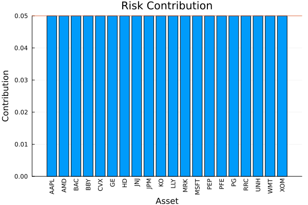
And the increasing-budget portfolio:
plot_risk_contribution(rf, res_inc, rd)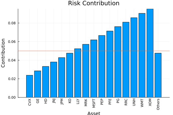
3. Relaxed risk budgeting
RelaxedRiskBudgeting (RRB) replaces the non-convex risk-parity constraint with a second-order-cone relaxation. It needs neither a logarithm nor integer variables, so it is cheaper to solve — useful at scale. It is variance-specific (the SOC is built on the Cholesky factor of the covariance), so it takes no r. Three variants trade exactness for regularisation: BasicRelaxedRiskBudgeting, RegularisedRelaxedRiskBudgeting, and RegularisedPenalisedRelaxedRiskBudgeting.
Being a relaxation, RRB does not adhere to the target risk budget as tightly as the exact log-barrier or mixed-integer formulations of section 2 — in pathological cases (ill-conditioned covariance, extreme budgets) the realised contributions can deviate noticeably. In exchange, the convex SOC formulation composes cleanly with additional constraints, making it the friendlier choice when the risk budget is one objective among several rather than a hard requirement. Reach for RiskBudgeting when strict adherence is essential.
rba_eq = AssetRiskBudgeting(; rkb = RiskBudget(; val = fill(1.0, N)))
rrb_basic = RelaxedRiskBudgeting(; opt = opt, rba = rba_eq,
                                 alg = BasicRelaxedRiskBudgeting())
rrb_reg = RelaxedRiskBudgeting(; opt = opt, rba = rba_eq,
                               alg = RegularisedRelaxedRiskBudgeting())
res_b, res_r = optimise(rrb_basic), optimise(rrb_reg)
(RiskBudgetingResult
jr ┼ JuMPOptimisationResult
│ pa ┼ ProcessedJuMPOptimiserAttributes
│ │ pr ┼ LowOrderPrior
│ │ │ X ┼ 252×20 Matrix{Float64}
│ │ │ mu ┼ 20-element Vector{Float64}
│ │ │ sigma ┼ 20×20 Matrix{Float64}
│ │ │ chol ┼ nothing
│ │ │ w ┼ nothing
│ │ │ ens ┼ nothing
│ │ │ kld ┼ nothing
│ │ │ ow ┼ nothing
│ │ │ rr ┼ nothing
│ │ │ f_mu ┼ nothing
│ │ │ f_sigma ┼ nothing
│ │ │ f_w ┴ nothing
│ │ wb ┼ WeightBounds
│ │ │ lb ┼ 20-element StepRangeLen{Float64, Base.TwicePrecision{Float64}, Base.TwicePrecision{Float64}, Int64}
│ │ │ ub ┴ 20-element StepRangeLen{Float64, Base.TwicePrecision{Float64}, Base.TwicePrecision{Float64}, Int64}
│ │ lt ┼ nothing
│ │ st ┼ nothing
│ │ lcsr ┼ nothing
│ │ ctr ┼ nothing
│ │ gcardr ┼ nothing
│ │ sgcardr ┼ nothing
│ │ smtx ┼ nothing
│ │ sgmtx ┼ nothing
│ │ slt ┼ nothing
│ │ sst ┼ nothing
│ │ sglt ┼ nothing
│ │ sgst ┼ nothing
│ │ tn ┼ nothing
│ │ fees ┼ nothing
│ │ plr ┼ nothing
│ │ ret ┼ ArithmeticReturn
│ │ │ ucs ┼ nothing
│ │ │ lb ┼ nothing
│ │ │ mu ┴ 20-element Vector{Float64}
│ retcode ┼ OptimisationSuccess
│ │ res ┴ Dict{Any, Any}: Dict{Any, Any}()
│ sol ┼ JuMPOptimisationSolution
│ │ w ┴ 20-element Vector{Float64}
│ model ┼ A JuMP Model
│ │ ├ solver: Clarabel
│ │ ├ objective_sense: MIN_SENSE
│ │ │ └ objective_function_type: AffExpr
│ │ ├ num_variables: 42
│ │ ├ num_constraints: 47
│ │ │ ├ AffExpr in MOI.EqualTo{Float64}: 1
│ │ │ ├ Vector{AffExpr} in MOI.Zeros: 1
│ │ │ ├ Vector{AffExpr} in MOI.Nonnegatives: 1
│ │ │ ├ Vector{AffExpr} in MOI.Nonpositives: 1
│ │ │ ├ Vector{AffExpr} in MOI.SecondOrderCone: 21
│ │ │ └ VariableRef in MOI.GreaterThan{Float64}: 22
│ │ └ Names registered in the model
│ │ └ :bgt, :cbasic_rrp, :crrp, :crrp_soc, :gamma, :k, :lw, :obj_expr, :psi, :ret, :risk, :sc, :so, :w, :w_lb, :w_ub, :zeta
prb ┼ ProcessedAssetRiskBudgetingAttributes
│ rkb ┼ RiskBudget
│ │ val ┴ 20-element Vector{Float64}
fb ┴ nothing
, RiskBudgetingResult
jr ┼ JuMPOptimisationResult
│ pa ┼ ProcessedJuMPOptimiserAttributes
│ │ pr ┼ LowOrderPrior
│ │ │ X ┼ 252×20 Matrix{Float64}
│ │ │ mu ┼ 20-element Vector{Float64}
│ │ │ sigma ┼ 20×20 Matrix{Float64}
│ │ │ chol ┼ nothing
│ │ │ w ┼ nothing
│ │ │ ens ┼ nothing
│ │ │ kld ┼ nothing
│ │ │ ow ┼ nothing
│ │ │ rr ┼ nothing
│ │ │ f_mu ┼ nothing
│ │ │ f_sigma ┼ nothing
│ │ │ f_w ┴ nothing
│ │ wb ┼ WeightBounds
│ │ │ lb ┼ 20-element StepRangeLen{Float64, Base.TwicePrecision{Float64}, Base.TwicePrecision{Float64}, Int64}
│ │ │ ub ┴ 20-element StepRangeLen{Float64, Base.TwicePrecision{Float64}, Base.TwicePrecision{Float64}, Int64}
│ │ lt ┼ nothing
│ │ st ┼ nothing
│ │ lcsr ┼ nothing
│ │ ctr ┼ nothing
│ │ gcardr ┼ nothing
│ │ sgcardr ┼ nothing
│ │ smtx ┼ nothing
│ │ sgmtx ┼ nothing
│ │ slt ┼ nothing
│ │ sst ┼ nothing
│ │ sglt ┼ nothing
│ │ sgst ┼ nothing
│ │ tn ┼ nothing
│ │ fees ┼ nothing
│ │ plr ┼ nothing
│ │ ret ┼ ArithmeticReturn
│ │ │ ucs ┼ nothing
│ │ │ lb ┼ nothing
│ │ │ mu ┴ 20-element Vector{Float64}
│ retcode ┼ OptimisationSuccess
│ │ res ┴ Dict{Any, Any}: Dict{Any, Any}()
│ sol ┼ JuMPOptimisationSolution
│ │ w ┴ 20-element Vector{Float64}
│ model ┼ A JuMP Model
│ │ ├ solver: Clarabel
│ │ ├ objective_sense: MIN_SENSE
│ │ │ └ objective_function_type: AffExpr
│ │ ├ num_variables: 43
│ │ ├ num_constraints: 49
│ │ │ ├ AffExpr in MOI.EqualTo{Float64}: 1
│ │ │ ├ Vector{AffExpr} in MOI.Zeros: 1
│ │ │ ├ Vector{AffExpr} in MOI.Nonnegatives: 1
│ │ │ ├ Vector{AffExpr} in MOI.Nonpositives: 1
│ │ │ ├ Vector{AffExpr} in MOI.SecondOrderCone: 22
│ │ │ └ VariableRef in MOI.GreaterThan{Float64}: 23
│ │ └ Names registered in the model
│ │ └ :bgt, :creg_rrp_soc_1, :creg_rrp_soc_2, :crrp, :crrp_soc, :gamma, :k, :lw, :obj_expr, :psi, :ret, :rho, :risk, :sc, :so, :w, :w_lb, :w_ub, :zeta
prb ┼ ProcessedAssetRiskBudgetingAttributes
│ rkb ┼ RiskBudget
│ │ val ┴ 20-element Vector{Float64}
fb ┴ nothing
)Comparing the relaxed solutions against the exact log-barrier ERC of section 2 shows the price of the relaxation: on this dataset the relaxed portfolios are noticeably more concentrated than the exact ERC, so the realised risk contributions spread away from the flat
rc_b = risk_contribution(rf, res_b.w, pr.X);
rc_b ./= sum(rc_b);
rc_r = risk_contribution(rf, res_r.w, pr.X);
rc_r ./= sum(rc_r);

pretty_table(DataFrame(; :assets => rd.nx, Symbol("Log ERC risk") => rc_eq,
                       Symbol("Basic RRB risk") => rc_b,
                       Symbol("Regularised RRB risk") => rc_r); formatters = [resfmt])
┌────────┬──────────────┬────────────────┬──────────────────────┐
│ assets │ Log ERC risk │ Basic RRB risk │ Regularised RRB risk │
│ String │ Float64 │ Float64 │ Float64 │
├────────┼──────────────┼────────────────┼──────────────────────┤
│ AAPL │ 5.0 % │ 2.965 % │ 1.963 % │
│ AMD │ 5.0 % │ 2.965 % │ 1.963 % │
│ BAC │ 5.0 % │ 2.965 % │ 1.963 % │
│ BBY │ 5.0 % │ 2.965 % │ 1.963 % │
│ CVX │ 5.0 % │ 2.989 % │ 4.235 % │
│ GE │ 5.0 % │ 2.965 % │ 1.963 % │
│ HD │ 5.0 % │ 2.965 % │ 1.963 % │
│ JNJ │ 5.0 % │ 27.581 % │ 31.471 % │
│ JPM │ 5.0 % │ 2.965 % │ 1.963 % │
│ KO │ 5.0 % │ 3.906 % │ 7.105 % │
│ LLY │ 5.0 % │ 2.965 % │ 1.963 % │
│ MRK │ 5.0 % │ 13.356 % │ 15.168 % │
│ MSFT │ 5.0 % │ 2.965 % │ 1.963 % │
│ PEP │ 5.0 % │ 2.965 % │ 4.341 % │
│ PFE │ 5.0 % │ 2.965 % │ 1.963 % │
│ ⋮ │ ⋮ │ ⋮ │ ⋮ │
└────────┴──────────────┴────────────────┴──────────────────────┘
5 rows omitted4. Factor risk budgeting
FactorRiskBudgeting allocates risk across factors rather than assets, via a regression of asset returns onto factor returns. It needs the factor returns, but not the factor prior so we should use use a EmpiricalPrior.
F = TimeArray(CSV.File(joinpath(@__DIR__, "..", "Factors.csv.gz")); timestamp = :Date)[(end - 252):end]
rdf = prices_to_returns(X, F)
prf = prior(EmpiricalPrior(), rdf)
optf = JuMPOptimiser(; pe = prf, slv = slv)
Nf = length(rdf.nf)

# Equal risk contribution across factors.
frb = RiskBudgeting(; r = Variance(), opt = optf,
                    rba = FactorRiskBudgeting(; rkb = RiskBudget(; val = fill(1.0, Nf))))
RiskBudgeting
opt ┼ JuMPOptimiser
│ pe ┼ LowOrderPrior
│ │ X ┼ 252×20 Matrix{Float64}
│ │ mu ┼ 20-element Vector{Float64}
│ │ sigma ┼ 20×20 Matrix{Float64}
│ │ chol ┼ nothing
│ │ w ┼ nothing
│ │ ens ┼ nothing
│ │ kld ┼ nothing
│ │ ow ┼ nothing
│ │ rr ┼ nothing
│ │ f_mu ┼ nothing
│ │ f_sigma ┼ nothing
│ │ f_w ┴ nothing
│ slv ┼ Solver
│ │ name ┼ Symbol: :clarabel
│ │ solver ┼ UnionAll: Clarabel.MOIwrapper.Optimizer
│ │ settings ┼ Dict{String, Bool}: Dict{String, Bool}("verbose" => 0)
│ │ check_sol ┼ @NamedTuple{allow_local::Bool, allow_almost::Bool}: (allow_local = true, allow_almost = true)
│ │ add_bridges ┴ Bool: true
│ wb ┼ WeightBounds
│ │ lb ┼ Float64: 0.0
│ │ ub ┴ Float64: 1.0
│ bgt ┼ Float64: 1.0
│ sbgt ┼ nothing
│ lt ┼ nothing
│ st ┼ nothing
│ lcse ┼ nothing
│ cte ┼ nothing
│ gcarde ┼ nothing
│ sgcarde ┼ nothing
│ smtx ┼ nothing
│ sgmtx ┼ nothing
│ slt ┼ nothing
│ sst ┼ nothing
│ sglt ┼ nothing
│ sgst ┼ nothing
│ tn ┼ nothing
│ fees ┼ nothing
│ sets ┼ nothing
│ tr ┼ nothing
│ ple ┼ nothing
│ ret ┼ ArithmeticReturn
│ │ ucs ┼ nothing
│ │ lb ┼ nothing
│ │ mu ┴ nothing
│ sca ┼ SumScalariser()
│ ccnt ┼ nothing
│ cobj ┼ nothing
│ sc ┼ Int64: 1
│ so ┼ Int64: 1
│ ss ┼ nothing
│ card ┼ nothing
│ scard ┼ nothing
│ wn2 ┼ nothing
│ wnp ┼ nothing
│ wninf ┼ nothing
│ l1 ┼ nothing
│ l2 ┼ nothing
│ linf ┼ nothing
│ lp ┼ nothing
│ brt ┼ Bool: false
│ cle_pr ┼ Bool: true
│ strict ┴ Bool: false
r ┼ Variance
│ settings ┼ RiskMeasureSettings
│ │ scale ┼ Float64: 1.0
│ │ ub ┼ nothing
│ │ rke ┴ Bool: true
│ sigma ┼ nothing
│ chol ┼ nothing
│ rc ┼ nothing
│ alg ┴ SquaredSOCRiskExpr()
rba ┼ FactorRiskBudgeting
│ re ┼ StepwiseRegression
│ │ crit ┼ PValue
│ │ │ t ┴ Float64: 0.05
│ │ alg ┼ ForwardSelection()
│ │ tgt ┼ LinearModel
│ │ │ kwargs ┴ @NamedTuple{}: NamedTuple()
│ rkb ┼ RiskBudget
│ │ val ┴ Vector{Float64}: [1.0, 1.0, 1.0, 1.0, 1.0]
│ sets ┼ nothing
│ flag ┴ Bool: true
wi ┼ nothing
fb ┴ nothingBecause re here is a regression estimator (StepwiseRegression by default), the factor model has to be fit while building the model, so the returns data must be passed to optimise even though the prior is precomputed. (If you instead pass a precomputed Regression result as re, no data is needed — and a clear error tells you if you missed passing rd when it's required.)
res_frb = optimise(frb, rdf)RiskBudgetingResult
jr ┼ JuMPOptimisationResult
│ pa ┼ ProcessedJuMPOptimiserAttributes
│ │ pr ┼ LowOrderPrior
│ │ │ X ┼ 252×20 Matrix{Float64}
│ │ │ mu ┼ 20-element Vector{Float64}
│ │ │ sigma ┼ 20×20 Matrix{Float64}
│ │ │ chol ┼ nothing
│ │ │ w ┼ nothing
│ │ │ ens ┼ nothing
│ │ │ kld ┼ nothing
│ │ │ ow ┼ nothing
│ │ │ rr ┼ nothing
│ │ │ f_mu ┼ nothing
│ │ │ f_sigma ┼ nothing
│ │ │ f_w ┴ nothing
│ │ wb ┼ WeightBounds
│ │ │ lb ┼ 20-element StepRangeLen{Float64, Base.TwicePrecision{Float64}, Base.TwicePrecision{Float64}, Int64}
│ │ │ ub ┴ 20-element StepRangeLen{Float64, Base.TwicePrecision{Float64}, Base.TwicePrecision{Float64}, Int64}
│ │ lt ┼ nothing
│ │ st ┼ nothing
│ │ lcsr ┼ nothing
│ │ ctr ┼ nothing
│ │ gcardr ┼ nothing
│ │ sgcardr ┼ nothing
│ │ smtx ┼ nothing
│ │ sgmtx ┼ nothing
│ │ slt ┼ nothing
│ │ sst ┼ nothing
│ │ sglt ┼ nothing
│ │ sgst ┼ nothing
│ │ tn ┼ nothing
│ │ fees ┼ nothing
│ │ plr ┼ nothing
│ │ ret ┼ ArithmeticReturn
│ │ │ ucs ┼ nothing
│ │ │ lb ┼ nothing
│ │ │ mu ┴ 20-element Vector{Float64}
│ retcode ┼ OptimisationSuccess
│ │ res ┴ Dict{Any, Any}: Dict{Any, Any}()
│ sol ┼ JuMPOptimisationSolution
│ │ w ┴ 20-element Vector{Float64}
│ model ┼ A JuMP Model
│ │ ├ solver: Clarabel
│ │ ├ objective_sense: MIN_SENSE
│ │ │ └ objective_function_type: QuadExpr
│ │ ├ num_variables: 27
│ │ ├ num_constraints: 10
│ │ │ ├ AffExpr in MOI.EqualTo{Float64}: 1
│ │ │ ├ AffExpr in MOI.GreaterThan{Float64}: 1
│ │ │ ├ Vector{AffExpr} in MOI.Nonnegatives: 1
│ │ │ ├ Vector{AffExpr} in MOI.Nonpositives: 1
│ │ │ ├ Vector{AffExpr} in MOI.SecondOrderCone: 1
│ │ │ └ Vector{AffExpr} in MOI.ExponentialCone: 5
│ │ └ Names registered in the model
│ │ └ :G, :bgt, :clog_w, :crkb, :dev_1, :dev_1_soc, :k, :log_w, :lw, :obj_expr, :ret, :risk, :risk_vec, :sc, :so, :variance_flag, :variance_risk_1, :w, :w1, :w2, :w_lb, :w_ub
prb ┼ ProcessedFactorRiskBudgetingAttributes
│ rkb ┼ RiskBudget
│ │ val ┴ Vector{Float64}: [1.0, 1.0, 1.0, 1.0, 1.0]
│ b1 ┼ 20×5 Matrix{Float64}
│ rr ┼ Regression
│ │ M ┼ 20×5 SubArray{Float64, 2, Matrix{Float64}, Tuple{Base.Slice{Base.OneTo{Int64}}, UnitRange{Int64}}, true}
│ │ L ┼ 20×5 SubArray{Float64, 2, Matrix{Float64}, Tuple{Base.Slice{Base.OneTo{Int64}}, UnitRange{Int64}}, true}
│ │ b ┴ 20-element SubArray{Float64, 1, Matrix{Float64}, Tuple{Base.Slice{Base.OneTo{Int64}}, Int64}, true}
fb ┴ nothingThe factor risk contributions (the trailing entry is the intercept/idiosyncratic term) cluster near the equal
rfk = factory(Variance(), prf)
frc = factor_risk_contribution(rfk, res_frb.w, prf.X; rd = rdf)
frc ./= sum(frc)

pretty_table(DataFrame(; :factor => [rdf.nf; "Intercept"], :risk => frc);
             formatters = [resfmt])

plot_factor_risk_contribution(rfk, res_frb, rdf)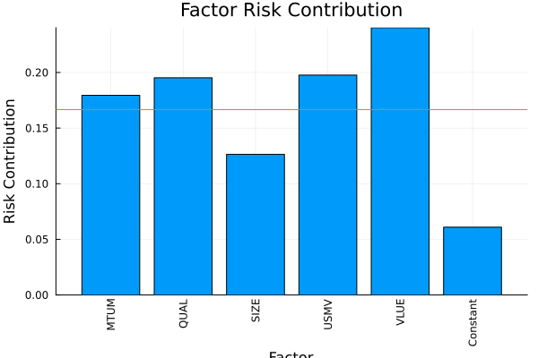
Summary
Risk budgeting targets a distribution of risk rather than a return/risk trade-off:
AssetRiskBudgetingspreads risk across assets — equal budgets give the ERC portfolio, arbitrary budgets express convictions about where risk should sit.RelaxedRiskBudgetingis the cheaper convex alternative; verify the realised contributions, as the relaxation need not reproduce exact risk parity.FactorRiskBudgetingbudgets risk across factors instead of assets, at the cost of needing the returns data at optimise time.
This page was generated using Literate.jl.