
The source files can be found in examples/.
Efficient frontier
A single MeanRisk objective returns one portfolio. The efficient frontier is the whole curve: the set of portfolios that earn the most return for each level of risk (equivalently, that take the least risk for each level of return). Instead of committing to one risk/return point up front, you trace the entire trade-off and choose by eye, hand it to a stakeholder, or feed the sweep to a downstream selection rule.
This example does three things the MeanRisk objectives page does not. First, it shows the frontier traced from both directions — minimising risk at a return floor, and maximising return at a risk ceiling — and that they recover the same curve. Second, it introduces the Frontier helper, which computes the sweep bounds automatically. Third, it contrasts the extreme MeanRisk frontier with the centred frontier produced by NearOptimalCentering, which trades a sliver of optimality for a more diversified, stable allocation at every point.
When to reach for this
Reach for an efficient frontier when you do not want to commit to a single risk/return point up front — you want to see the whole trade-off curve and choose a portfolio by eye, hand it to a stakeholder, or feed the sweep to a downstream selection rule. It is the natural next step once you understand the MeanRisk objectives: instead of one objective value, you sweep the risk/return frontier. For more than two competing criteria, see the Pareto surface example.
using PortfolioOptimisers, PrettyTables
# Format for pretty tables.
tsfmt = (v, i, j) -> begin
    if j == 1
        return Date(v)
    else
        return v
    end
end;
resfmt = (v, i, j) -> begin
    if j == 1
        return v
    else
        return isa(v, Number) ? "$(round(v*100, digits=3)) %" : v
    end
end;
1. ReturnsResult data
We use the same S&P 500 slice as the other optimiser examples.
using CSV, TimeSeries, DataFrames

X = TimeArray(CSV.File(joinpath(@__DIR__, "..", "SP500.csv.gz")); timestamp = :Date)[(end - 252):end]
pretty_table(X[(end - 5):end]; formatters = [tsfmt])

# Compute the returns
rd = prices_to_returns(X)
ReturnsResult
nx ┼ 20-element Vector{String}
X ┼ 252×20 Matrix{Float64}
nf ┼ nothing
F ┼ nothing
nb ┼ nothing
B ┼ nothing
ts ┼ 252-element Vector{Date}
iv ┼ nothing
ivpa ┴ nothing2. Two directions, four combinations
There are two mutually exclusive ways to trace a frontier:
Minimise risk subject to a lower bound on return — sweep the return floor upward.
Maximise return subject to an upper bound on risk — sweep the risk ceiling upward.
Each bound can be supplied explicitly (a range of numbers you pick) or as a Frontier object, which inspects the problem, finds the feasible extremes, and lays out the sweep for you. That is the four combinations — two directions × explicit/automatic bounds — and they all have their uses. The two directions trace the same curve; the choice is about which quantity is more natural to pin in your problem.
We will use the ConditionalValueatRisk measure throughout, and precompute the prior once so every optimisation reuses it. Since we run many optimisations and cannot assume a single solver configuration converges at every point, we pass a vector of solver settings and let the optimiser fall back through them.
using Clarabel
slv = [Solver(; name = :clarabel1, solver = Clarabel.Optimizer,
              settings = Dict("verbose" => false),
              check_sol = (; allow_local = true, allow_almost = true)),
       Solver(; name = :clarabel2, solver = Clarabel.Optimizer,
              settings = Dict("verbose" => false, "max_step_fraction" => 0.75),
              check_sol = (; allow_local = true, allow_almost = true))]

r = ConditionalValueatRisk()
pr = prior(EmpiricalPrior(), rd)
rf = 4.2 / 100 / 2520.0001666666666666667Direction A — minimise risk along a return floor
We minimise CVaR (the default objective) while a Frontier sweeps the return lower bound, giving a 30-point frontier. The lower bound lives on the return side, so it is set through ArithmeticReturn's lb.
optA = JuMPOptimiser(; pe = pr, slv = slv,
                     ret = ArithmeticReturn(; lb = Frontier(; N = 30)))
resA = optimise(MeanRisk(; opt = optA, r = r))
MeanRiskResult
jr ┼ JuMPOptimisationResult
│ pa ┼ ProcessedJuMPOptimiserAttributes
│ │ pr ┼ LowOrderPrior
│ │ │ X ┼ 252×20 Matrix{Float64}
│ │ │ mu ┼ 20-element Vector{Float64}
│ │ │ sigma ┼ 20×20 Matrix{Float64}
│ │ │ chol ┼ nothing
│ │ │ w ┼ nothing
│ │ │ ens ┼ nothing
│ │ │ kld ┼ nothing
│ │ │ ow ┼ nothing
│ │ │ rr ┼ nothing
│ │ │ f_mu ┼ nothing
│ │ │ f_sigma ┼ nothing
│ │ │ f_w ┴ nothing
│ │ wb ┼ WeightBounds
│ │ │ lb ┼ 20-element StepRangeLen{Float64, Base.TwicePrecision{Float64}, Base.TwicePrecision{Float64}, Int64}
│ │ │ ub ┴ 20-element StepRangeLen{Float64, Base.TwicePrecision{Float64}, Base.TwicePrecision{Float64}, Int64}
│ │ lt ┼ nothing
│ │ st ┼ nothing
│ │ lcsr ┼ nothing
│ │ ctr ┼ nothing
│ │ gcardr ┼ nothing
│ │ sgcardr ┼ nothing
│ │ smtx ┼ nothing
│ │ sgmtx ┼ nothing
│ │ slt ┼ nothing
│ │ sst ┼ nothing
│ │ sglt ┼ nothing
│ │ sgst ┼ nothing
│ │ tn ┼ nothing
│ │ fees ┼ nothing
│ │ plr ┼ nothing
│ │ ret ┼ ArithmeticReturn
│ │ │ ucs ┼ nothing
│ │ │ lb ┼ Frontier
│ │ │ │ N ┼ Int64: 30
│ │ │ │ factor ┼ Int64: 1
│ │ │ │ bound ┴ LinearBound()
│ │ │ mu ┴ 20-element Vector{Float64}
│ retcode ┼ 30-element Vector{OptimisationSuccess}
│ │ OptimisationSuccess ⋯
│ │ OptimisationSuccess ⋯
│ │ OptimisationSuccess ⋯
│ │ OptimisationSuccess ⋯
│ │ OptimisationSuccess ⋯
│ │ OptimisationSuccess ⋯
│ │ OptimisationSuccess ⋯
│ │ OptimisationSuccess ⋯
│ │ OptimisationSuccess ⋯
│ │ OptimisationSuccess ⋯
│ │ OptimisationSuccess ⋯
│ │ OptimisationSuccess ⋯
│ │ OptimisationSuccess ⋯
│ │ OptimisationSuccess ⋯
│ │ OptimisationSuccess ⋯
│ │ OptimisationSuccess ⋯
│ │ OptimisationSuccess ⋯
│ │ OptimisationSuccess ⋯
│ │ OptimisationSuccess ⋯
│ │ OptimisationSuccess ⋯
│ │ OptimisationSuccess ⋯
│ │ OptimisationSuccess ⋯
│ │ OptimisationSuccess ⋯
│ │ OptimisationSuccess ⋯
│ │ OptimisationSuccess ⋯
│ │ OptimisationSuccess ⋯
│ │ OptimisationSuccess ⋯
│ │ OptimisationSuccess ⋯
│ │ OptimisationSuccess ⋯
│ │ OptimisationSuccess ⋯
│ sol ┼ 30-element Vector{JuMPOptimisationSolution}
│ │ JuMPOptimisationSolution ⋯
│ │ JuMPOptimisationSolution ⋯
│ │ JuMPOptimisationSolution ⋯
│ │ JuMPOptimisationSolution ⋯
│ │ JuMPOptimisationSolution ⋯
│ │ JuMPOptimisationSolution ⋯
│ │ JuMPOptimisationSolution ⋯
│ │ JuMPOptimisationSolution ⋯
│ │ JuMPOptimisationSolution ⋯
│ │ JuMPOptimisationSolution ⋯
│ │ JuMPOptimisationSolution ⋯
│ │ JuMPOptimisationSolution ⋯
│ │ JuMPOptimisationSolution ⋯
│ │ JuMPOptimisationSolution ⋯
│ │ JuMPOptimisationSolution ⋯
│ │ JuMPOptimisationSolution ⋯
│ │ JuMPOptimisationSolution ⋯
│ │ JuMPOptimisationSolution ⋯
│ │ JuMPOptimisationSolution ⋯
│ │ JuMPOptimisationSolution ⋯
│ │ JuMPOptimisationSolution ⋯
│ │ JuMPOptimisationSolution ⋯
│ │ JuMPOptimisationSolution ⋯
│ │ JuMPOptimisationSolution ⋯
│ │ JuMPOptimisationSolution ⋯
│ │ JuMPOptimisationSolution ⋯
│ │ JuMPOptimisationSolution ⋯
│ │ JuMPOptimisationSolution ⋯
│ │ JuMPOptimisationSolution ⋯
│ │ JuMPOptimisationSolution ⋯
│ model ┼ A JuMP Model
│ │ ├ solver: Clarabel
│ │ ├ objective_sense: MIN_SENSE
│ │ │ └ objective_function_type: AffExpr
│ │ ├ num_variables: 274
│ │ ├ num_constraints: 258
│ │ │ ├ AffExpr in MOI.EqualTo{Float64}: 1
│ │ │ ├ AffExpr in MOI.GreaterThan{Float64}: 1
│ │ │ ├ Vector{AffExpr} in MOI.Nonnegatives: 2
│ │ │ ├ Vector{AffExpr} in MOI.Nonpositives: 1
│ │ │ ├ VariableRef in MOI.GreaterThan{Float64}: 252
│ │ │ └ VariableRef in MOI.Parameter{Float64}: 1
│ │ └ Names registered in the model
│ │ └ :X, :bgt, :ccvar_1, :cvar_risk_1, :k, :lw, :net_X, :obj_expr, :ret, :ret_frontier, :ret_lb, :ret_lb_var, :risk, :risk_vec, :sc, :so, :var_1, :w, :w_lb, :w_ub, :z_cvar_1
fb ┴ nothingretcode and sol are now vectors — one entry per frontier point. We had no warnings about failed optimisations, but let's confirm every point solved.
all(x -> isa(x, OptimisationSuccess), resA.retcode)trueThe weights evolve smoothly from the low-risk end (diversified) toward the high-return end (concentrated) as we walk up the frontier.
pretty_table(DataFrame([rd.nx hcat(resA.w...)], Symbol.([:assets; 1:30]));
             formatters = [resfmt])
┌────────┬──────────┬──────────┬──────────┬──────────┬──────────┬──────────┬────
│ assets │ 1 │ 2 │ 3 │ 4 │ 5 │ 6 │ ⋯
│ Any │ Any │ Any │ Any │ Any │ Any │ Any │ ⋯
├────────┼──────────┼──────────┼──────────┼──────────┼──────────┼──────────┼────
│ AAPL │ 0.0 % │ 0.0 % │ 0.0 % │ 0.0 % │ 0.0 % │ 0.0 % │ ⋯
│ AMD │ 0.0 % │ 0.0 % │ 0.0 % │ 0.0 % │ 0.0 % │ 0.0 % │ ⋯
│ BAC │ 0.0 % │ 0.0 % │ 0.0 % │ 0.0 % │ 0.0 % │ 0.0 % │ ⋯
│ BBY │ 0.0 % │ 0.0 % │ 0.0 % │ 0.0 % │ 0.0 % │ 0.0 % │ ⋯
│ CVX │ 13.167 % │ 12.757 % │ 9.552 % │ 3.037 % │ 1.821 % │ 0.159 % │ ⋯
│ GE │ 0.0 % │ 0.0 % │ 0.0 % │ 0.0 % │ 0.0 % │ 0.0 % │ ⋯
│ HD │ 0.0 % │ 0.0 % │ 0.0 % │ 0.0 % │ 0.0 % │ 0.0 % │ ⋯
│ JNJ │ 45.342 % │ 40.238 % │ 37.261 % │ 32.596 % │ 29.384 % │ 26.772 % │ 2 ⋯
│ JPM │ 0.0 % │ 0.0 % │ 0.0 % │ 0.0 % │ 0.0 % │ 0.0 % │ ⋯
│ KO │ 13.285 % │ 14.244 % │ 14.767 % │ 18.327 % │ 17.772 % │ 17.332 % │ 1 ⋯
│ LLY │ 0.0 % │ 0.0 % │ 0.0 % │ 0.0 % │ 0.0 % │ 0.0 % │ ⋯
│ MRK │ 20.556 % │ 25.205 % │ 27.696 % │ 29.897 % │ 33.915 % │ 36.555 % │ 3 ⋯
│ MSFT │ 0.0 % │ 0.0 % │ 0.0 % │ 0.0 % │ 0.0 % │ 0.0 % │ ⋯
│ PEP │ 0.0 % │ 0.0 % │ 0.0 % │ 0.0 % │ 0.0 % │ 0.0 % │ ⋯
│ PFE │ 0.0 % │ 0.0 % │ 0.0 % │ 0.0 % │ 0.0 % │ 0.0 % │ ⋯
│ ⋮ │ ⋮ │ ⋮ │ ⋮ │ ⋮ │ ⋮ │ ⋮ │ ⋱
└────────┴──────────┴──────────┴──────────┴──────────┴──────────┴──────────┴────
24 columns and 5 rows omittedDirection B — maximise return under a risk ceiling
The dual route: maximise return while a Frontier sweeps an upper bound on CVaR. The bound now lives on the risk side, so it is attached to the risk measure through its RiskMeasureSettings. Everything else is identical.
optB = JuMPOptimiser(; pe = pr, slv = slv)
resB = optimise(MeanRisk(; opt = optB, obj = MaximumReturn(),
                         r = ConditionalValueatRisk(;
                                                    settings = RiskMeasureSettings(;
                                                                                   ub = Frontier(;
                                                                                                 N = 30)))))
all(x -> isa(x, OptimisationSuccess), resB.retcode)trueThe two directions trace the same trade-off curve. Computing the CVaR and the arithmetic return of each point lets us overlay them: the risk-floor sweep and the return-ceiling sweep land on top of one another (up to where the automatic bounds place their points).
rcvar = factory(ConditionalValueatRisk(), pr)
xs_A = [expected_risk(rcvar, w, pr.X) for w in resA.w]
ys_A = [expected_return(ArithmeticReturn(), w, pr) for w in resA.w]
xs_B = [expected_risk(rcvar, w, pr.X) for w in resB.w]
ys_B = [expected_return(ArithmeticReturn(), w, pr) for w in resB.w]

using StatsPlots, GraphRecipes

plot(xs_A, ys_A; seriestype = :scatter, marker = (:circle, 5),
     label = "Min risk | return floor", xlabel = "CVaR", ylabel = "Arithmetic return",
     title = "Same frontier from both directions")
plot!(xs_B, ys_B; seriestype = :scatter, marker = (:cross, 7),
      label = "Max return | risk ceiling")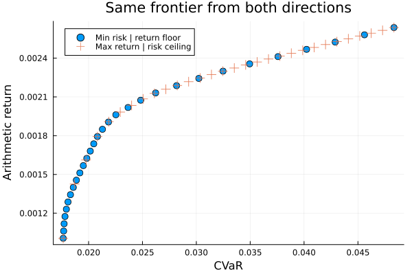
3. The MeanRisk frontier vs the NearOptimalCentering frontier
The frontier above is built from extreme points — each one exactly extremises the objective, and the high-return end loads heavily on a couple of names. NearOptimalCentering (NOC) traces a centred frontier instead: at each point it returns the portfolio at the analytic centre of the near-optimal neighbourhood rather than the corner. The result sits just inside the extreme frontier — slightly less optimal, noticeably more diversified and more stable to changes in the prior. (NOC's neighbourhood-centring behaviour is dissected on its own page; here we only use it as a frontier engine.)
NOC solves a harder problem than plain MeanRisk, so a single solver configuration can fail to converge. We give it a richer fallback vector with decreasing max_step_fraction.
slv_noc = [Solver(; name = Symbol("clarabel$i"), solver = Clarabel.Optimizer,
                  settings = Dict("verbose" => false, "max_step_fraction" => f),
                  check_sol = (; allow_local = true, allow_almost = true))
           for (i, f) in enumerate((0.99, 0.95, 0.9, 0.85, 0.8, 0.75, 0.7))]
7-element Vector{Solver{Symbol, UnionAll, Dict{String, Real}, @NamedTuple{allow_local::Bool, allow_almost::Bool}, Bool}}:
Solver
name ┼ Symbol: :clarabel1
solver ┼ UnionAll: Clarabel.MOIwrapper.Optimizer
settings ┼ Dict{String, Real}: Dict{String, Real}("verbose" => false, "max_step_fraction" => 0.99)
check_sol ┼ @NamedTuple{allow_local::Bool, allow_almost::Bool}: (allow_local = true, allow_almost = true)
add_bridges ┴ Bool: true
Solver
name ┼ Symbol: :clarabel2
solver ┼ UnionAll: Clarabel.MOIwrapper.Optimizer
settings ┼ Dict{String, Real}: Dict{String, Real}("verbose" => false, "max_step_fraction" => 0.95)
check_sol ┼ @NamedTuple{allow_local::Bool, allow_almost::Bool}: (allow_local = true, allow_almost = true)
add_bridges ┴ Bool: true
Solver
name ┼ Symbol: :clarabel3
solver ┼ UnionAll: Clarabel.MOIwrapper.Optimizer
settings ┼ Dict{String, Real}: Dict{String, Real}("verbose" => false, "max_step_fraction" => 0.9)
check_sol ┼ @NamedTuple{allow_local::Bool, allow_almost::Bool}: (allow_local = true, allow_almost = true)
add_bridges ┴ Bool: true
Solver
name ┼ Symbol: :clarabel4
solver ┼ UnionAll: Clarabel.MOIwrapper.Optimizer
settings ┼ Dict{String, Real}: Dict{String, Real}("verbose" => false, "max_step_fraction" => 0.85)
check_sol ┼ @NamedTuple{allow_local::Bool, allow_almost::Bool}: (allow_local = true, allow_almost = true)
add_bridges ┴ Bool: true
Solver
name ┼ Symbol: :clarabel5
solver ┼ UnionAll: Clarabel.MOIwrapper.Optimizer
settings ┼ Dict{String, Real}: Dict{String, Real}("verbose" => false, "max_step_fraction" => 0.8)
check_sol ┼ @NamedTuple{allow_local::Bool, allow_almost::Bool}: (allow_local = true, allow_almost = true)
add_bridges ┴ Bool: true
Solver
name ┼ Symbol: :clarabel6
solver ┼ UnionAll: Clarabel.MOIwrapper.Optimizer
settings ┼ Dict{String, Real}: Dict{String, Real}("verbose" => false, "max_step_fraction" => 0.75)
check_sol ┼ @NamedTuple{allow_local::Bool, allow_almost::Bool}: (allow_local = true, allow_almost = true)
add_bridges ┴ Bool: true
Solver
name ┼ Symbol: :clarabel7
solver ┼ UnionAll: Clarabel.MOIwrapper.Optimizer
settings ┼ Dict{String, Real}: Dict{String, Real}("verbose" => false, "max_step_fraction" => 0.7)
check_sol ┼ @NamedTuple{allow_local::Bool, allow_almost::Bool}: (allow_local = true, allow_almost = true)
add_bridges ┴ Bool: trueFor an apples-to-apples comparison we build both frontiers over the same 15-point return-floor sweep — only the optimiser changes.
ret15 = ArithmeticReturn(; lb = Frontier(; N = 15))
resM = optimise(MeanRisk(; opt = JuMPOptimiser(; pe = pr, slv = slv_noc, ret = ret15),
                         r = r))
resN = optimise(NearOptimalCentering(;
                                     opt = JuMPOptimiser(; pe = pr, slv = slv_noc,
                                                         ret = ret15), r = r))
NearOptimalCenteringResult
jr ┼ JuMPOptimisationResult
│ pa ┼ ProcessedJuMPOptimiserAttributes
│ │ pr ┼ LowOrderPrior
│ │ │ X ┼ 252×20 Matrix{Float64}
│ │ │ mu ┼ 20-element Vector{Float64}
│ │ │ sigma ┼ 20×20 Matrix{Float64}
│ │ │ chol ┼ nothing
│ │ │ w ┼ nothing
│ │ │ ens ┼ nothing
│ │ │ kld ┼ nothing
│ │ │ ow ┼ nothing
│ │ │ rr ┼ nothing
│ │ │ f_mu ┼ nothing
│ │ │ f_sigma ┼ nothing
│ │ │ f_w ┴ nothing
│ │ wb ┼ WeightBounds
│ │ │ lb ┼ 20-element StepRangeLen{Float64, Base.TwicePrecision{Float64}, Base.TwicePrecision{Float64}, Int64}
│ │ │ ub ┴ 20-element StepRangeLen{Float64, Base.TwicePrecision{Float64}, Base.TwicePrecision{Float64}, Int64}
│ │ lt ┼ nothing
│ │ st ┼ nothing
│ │ lcsr ┼ nothing
│ │ ctr ┼ nothing
│ │ gcardr ┼ nothing
│ │ sgcardr ┼ nothing
│ │ smtx ┼ nothing
│ │ sgmtx ┼ nothing
│ │ slt ┼ nothing
│ │ sst ┼ nothing
│ │ sglt ┼ nothing
│ │ sgst ┼ nothing
│ │ tn ┼ nothing
│ │ fees ┼ nothing
│ │ plr ┼ nothing
│ │ ret ┼ ArithmeticReturn
│ │ │ ucs ┼ nothing
│ │ │ lb ┼ nothing
│ │ │ mu ┴ 20-element Vector{Float64}
│ retcode ┼ OptimisationSuccess
│ │ res ┴ nothing
│ sol ┼ 15-element Vector{JuMPOptimisationSolution}
│ │ JuMPOptimisationSolution ⋯
│ │ JuMPOptimisationSolution ⋯
│ │ JuMPOptimisationSolution ⋯
│ │ JuMPOptimisationSolution ⋯
│ │ JuMPOptimisationSolution ⋯
│ │ JuMPOptimisationSolution ⋯
│ │ JuMPOptimisationSolution ⋯
│ │ JuMPOptimisationSolution ⋯
│ │ JuMPOptimisationSolution ⋯
│ │ JuMPOptimisationSolution ⋯
│ │ JuMPOptimisationSolution ⋯
│ │ JuMPOptimisationSolution ⋯
│ │ JuMPOptimisationSolution ⋯
│ │ JuMPOptimisationSolution ⋯
│ │ JuMPOptimisationSolution ⋯
│ model ┼ A JuMP Model
│ │ ├ solver: Clarabel
│ │ ├ objective_sense: MIN_SENSE
│ │ │ └ objective_function_type: AffExpr
│ │ ├ num_variables: 317
│ │ ├ num_constraints: 300
│ │ │ ├ AffExpr in MOI.EqualTo{Float64}: 1
│ │ │ ├ Vector{AffExpr} in MOI.Nonnegatives: 2
│ │ │ ├ Vector{AffExpr} in MOI.Nonpositives: 1
│ │ │ ├ Vector{AffExpr} in MOI.ExponentialCone: 42
│ │ │ ├ VariableRef in MOI.GreaterThan{Float64}: 252
│ │ │ └ VariableRef in MOI.Parameter{Float64}: 2
│ │ └ Names registered in the model
│ │ └ :X, :bgt, :ccvar_1, :clog_delta_w, :clog_ret, :clog_risk, :clog_w, :cvar_risk_1, :k, :log_delta_w, :log_ret, :log_risk, :log_w, :lw, :net_X, :noc_rk, :noc_rt, :obj_expr, :ret, :risk, :risk_vec, :sc, :so, :var_1, :w, :w_lb, :w_ub, :z_cvar_1
w_min_retcode ┼ OptimisationSuccess
│ res ┴ Dict{Any, Any}: Dict{Any, Any}()
w_opt_retcode ┼ 15-element Vector{OptimisationSuccess}
│ OptimisationSuccess ⋯
│ OptimisationSuccess ⋯
│ OptimisationSuccess ⋯
│ OptimisationSuccess ⋯
│ OptimisationSuccess ⋯
│ OptimisationSuccess ⋯
│ OptimisationSuccess ⋯
│ OptimisationSuccess ⋯
│ OptimisationSuccess ⋯
│ OptimisationSuccess ⋯
│ OptimisationSuccess ⋯
│ OptimisationSuccess ⋯
│ OptimisationSuccess ⋯
│ OptimisationSuccess ⋯
│ OptimisationSuccess ⋯
w_max_retcode ┼ OptimisationSuccess
│ res ┴ Dict{Any, Any}: Dict{Any, Any}()
noc_retcode ┼ 15-element Vector{OptimisationSuccess}
│ OptimisationSuccess ⋯
│ OptimisationSuccess ⋯
│ OptimisationSuccess ⋯
│ OptimisationSuccess ⋯
│ OptimisationSuccess ⋯
│ OptimisationSuccess ⋯
│ OptimisationSuccess ⋯
│ OptimisationSuccess ⋯
│ OptimisationSuccess ⋯
│ OptimisationSuccess ⋯
│ OptimisationSuccess ⋯
│ OptimisationSuccess ⋯
│ OptimisationSuccess ⋯
│ OptimisationSuccess ⋯
│ OptimisationSuccess ⋯
fb ┴ nothingNOC summarises its many internal MeanRisk solves into a single retcode; let's confirm success.
isa(resN.retcode, OptimisationSuccess)trueThe diversification difference is the point. We tabulate, at each frontier point, the largest single weight: NOC consistently holds a lower maximum weight — it fans the allocation out — except at the high-return end, where both frontiers are forced into the same return-maximising corner.
maxw(ws) = [round(maximum(w) * 100; digits = 1) for w in ws]
pretty_table(DataFrame("point" => 1:15, "MeanRisk max w %" => maxw(resM.w),
                       "NOC max w %" => maxw(resN.w));
             title = "Largest single weight along each frontier")
Largest single weight along each frontier
┌───────┬──────────────────┬─────────────┐
│ point │ MeanRisk max w % │ NOC max w % │
│ Int64 │ Float64 │ Float64 │
├───────┼──────────────────┼─────────────┤
│ 1 │ 45.3 │ 35.2 │
│ 2 │ 37.2 │ 34.5 │
│ 3 │ 34.5 │ 41.1 │
│ 4 │ 40.1 │ 43.2 │
│ 5 │ 46.9 │ 44.8 │
│ 6 │ 52.9 │ 45.2 │
│ 7 │ 59.0 │ 46.3 │
│ 8 │ 65.6 │ 46.5 │
│ 9 │ 71.6 │ 44.0 │
│ 10 │ 60.2 │ 46.1 │
│ 11 │ 51.9 │ 54.8 │
│ 12 │ 63.9 │ 65.8 │
│ 13 │ 75.9 │ 77.2 │
│ 14 │ 88.0 │ 87.6 │
│ 15 │ 100.0 │ 93.6 │
└───────┴──────────────────┴─────────────┘Plotted on the risk/return plane, the NOC frontier sits inside (to the upper-left of) the MeanRisk frontier: for a given return it accepts a little more CVaR, the price of sitting at the centre of the near-optimal region rather than at its edge.
xs_M = [expected_risk(rcvar, w, pr.X) for w in resM.w]
ys_M = [expected_return(ArithmeticReturn(), w, pr) for w in resM.w]
xs_N = [expected_risk(rcvar, w, pr.X) for w in resN.w]
ys_N = [expected_return(ArithmeticReturn(), w, pr) for w in resN.w]

plot(xs_M, ys_M; seriestype = :scatter, marker = (:circle, 5), label = "MeanRisk (extreme)",
     xlabel = "CVaR", ylabel = "Arithmetic return", title = "Extreme vs centred frontier")
plot!(xs_N, ys_N; seriestype = :scatter, marker = (:diamond, 6), label = "NOC (centred)")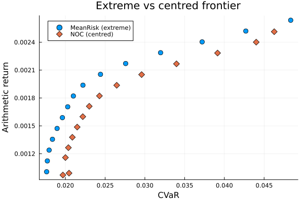
The composition along each frontier makes the same story visual: the MeanRisk frontier collapses onto a handful of names as it climbs, while the NOC frontier keeps more assets in play for longer.
plot_stacked_area_composition(resM.w, rd.nx)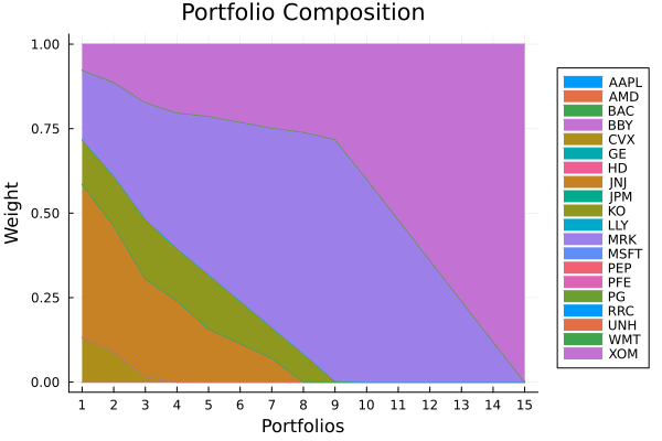
The same sweep under NOC — visibly more names carried up the frontier.
plot_stacked_area_composition(resN.w, rd.nx)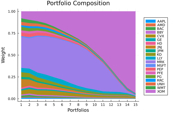
4. Visualising the frontier
The efficient frontier is a special case of a Pareto front, and plot_measures draws it on any pair of risk/return axes. There are optional keyword parameters for the risk measure on the X-axis, Y-axis, Z-axis, and colourbar. Here we put CVaR on the X-axis, the arithmetic return on the Y-axis, and colour by the risk-return ratio.
plot_measures(resA.w, resA.pr; x = r, y = ExpectedReturn(; rt = resA.ret),
              c = ExpectedReturnRiskRatio(; rt = resA.ret, rk = r, rf = rf),
              title = "Efficient Frontier", xlabel = "CVaR", ylabel = "Arithmetic Return",
              colorbar_title = "\nRisk/Return Ratio", right_margin = 6Plots.mm)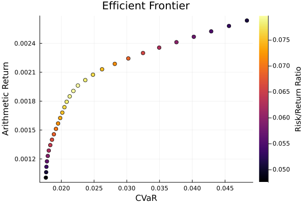
Because plot_measures works on any pair of measures, the same call plots arbitrary Pareto fronts — we can even use the ratio of two risk measures as the colourbar.
plot_measures(resA.w, resA.pr; x = r, y = ConditionalDrawdownatRisk(),
              c = RiskRatio(; r1 = ConditionalDrawdownatRisk(), r2 = r),
              title = "Pareto Front", xlabel = "CVaR", ylabel = "CDaR",
              colorbar_title = "\nCDaR/CVaR Ratio", right_margin = 6Plots.mm)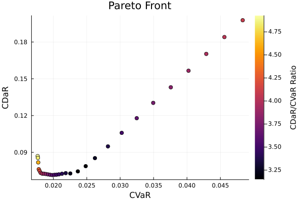
This page was generated using Literate.jl.