
The source files can be found in examples/.
Subset resampling and cross-validation
This example deepens the basic meta-optimiser walkthrough by focusing on two practical questions:
how stable are the out-of-sample predictions produced by a plain optimiser versus a meta-optimiser when we evaluate them with cross validation?
what does the efficient frontier look like when the optimiser is a meta-optimiser that resamples the universe before averaging the result?
We use MeanRisk as the benchmark and SubsetResampling as the meta- optimiser. The example also reuses the same clustering/prior setup as the standard meta- optimiser page so the allocations can be compared directly.
When to reach for this
Reach for subset resampling, and meta-optimisers generally, when a single full-universe fit feels brittle — when small changes in the estimation window swing the allocation, or when you want a portfolio averaged over many resampled universes rather than committed to one point estimate. Cross-validation here is the tool for checking that stability, not for producing the final portfolio.
using PortfolioOptimisers, PrettyTables, StableRNGs

resfmt = (v, i, j) -> begin
    if j == 1
        return v
    else
        return isa(v, Number) ? "$(round(v * 100, digits = 3)) %" : v
    end
end;
1. ReturnsResult data and shared ingredients
We use the same S&P 500 slice as the other optimiser examples. The shared prior and clustering are computed once and reused everywhere below.
using CSV, TimeSeries, DataFrames, Clarabel, Statistics

X = TimeArray(CSV.File(joinpath(@__DIR__, "..", "SP500.csv.gz")); timestamp = :Date)[(end - 252):end]
rd = prices_to_returns(X)

slv = [Solver(; name = :clarabel1, solver = Clarabel.Optimizer,
              settings = Dict("verbose" => false),
              check_sol = (; allow_local = true, allow_almost = true)),
       Solver(; name = :clarabel2, solver = Clarabel.Optimizer,
              settings = Dict("verbose" => false, "max_step_fraction" => 0.95),
              check_sol = (; allow_local = true, allow_almost = true)),
       Solver(; name = :clarabel3, solver = Clarabel.Optimizer,
              settings = Dict("verbose" => false, "max_step_fraction" => 0.9),
              check_sol = (; allow_local = true, allow_almost = true))]

pr = prior(EmpiricalPrior(), rd)
clr = clusterise(ClustersEstimator(; alg = DBHT()), pr.X)
jopti = JuMPOptimiser(; pe = pr, slv = slv)
jopto = JuMPOptimiser(; slv = slv)
JuMPOptimiser
pe ┼ EmpiricalPrior
│ ce ┼ PortfolioOptimisersCovariance
│ │ ce ┼ Covariance
│ │ │ me ┼ SimpleExpectedReturns
│ │ │ │ w ┴ nothing
│ │ │ ce ┼ GeneralCovariance
│ │ │ │ ce ┼ SimpleCovariance: SimpleCovariance(true)
│ │ │ │ w ┴ nothing
│ │ │ alg ┴ FullMoment()
│ │ mp ┼ MatrixProcessing
│ │ │ pdm ┼ Posdef
│ │ │ │ alg ┼ UnionAll: NearestCorrelationMatrix.Newton
│ │ │ │ kwargs ┴ @NamedTuple{}: NamedTuple()
│ │ │ dn ┼ nothing
│ │ │ dt ┼ nothing
│ │ │ alg ┼ nothing
│ │ │ order ┴ NTuple{4, Symbol}: (:pdm, :dn, :dt, :alg)
│ me ┼ SimpleExpectedReturns
│ │ w ┴ nothing
│ horizon ┴ nothing
slv ┼ 3-element Vector{Solver}
│ Solver ⋯
│ Solver ⋯
│ Solver ⋯
wb ┼ WeightBounds
│ lb ┼ Float64: 0.0
│ ub ┴ Float64: 1.0
bgt ┼ Float64: 1.0
sbgt ┼ nothing
lt ┼ nothing
st ┼ nothing
lcse ┼ nothing
cte ┼ nothing
gcarde ┼ nothing
sgcarde ┼ nothing
smtx ┼ nothing
sgmtx ┼ nothing
slt ┼ nothing
sst ┼ nothing
sglt ┼ nothing
sgst ┼ nothing
tn ┼ nothing
fees ┼ nothing
sets ┼ nothing
tr ┼ nothing
ple ┼ nothing
ret ┼ ArithmeticReturn
│ ucs ┼ nothing
│ lb ┼ nothing
│ mu ┴ nothing
sca ┼ SumScalariser()
ccnt ┼ nothing
cobj ┼ nothing
sc ┼ Int64: 1
so ┼ Int64: 1
ss ┼ nothing
card ┼ nothing
scard ┼ nothing
wn2 ┼ nothing
wnp ┼ nothing
wninf ┼ nothing
l1 ┼ nothing
l2 ┼ nothing
linf ┼ nothing
lp ┼ nothing
brt ┼ Bool: false
cle_pr ┼ Bool: true
strict ┴ Bool: false2. Reference allocations
We compute the plain minimum-variance portfolio and the three standard meta-optimisers. These are the same building blocks as the shorter overview example, but here we will reuse them for cross-validation and frontier comparisons.
res_bench = optimise(MeanRisk(; opt = JuMPOptimiser(; pe = pr, slv = slv)))

res_nco = optimise(NestedClustered(; pe = pr, cle = clr,
                                   opti = MeanRisk(; obj = MinimumRisk(), opt = jopti),
                                   opto = MeanRisk(; obj = MinimumRisk(), opt = jopto)), rd)

res_stk = optimise(Stacking(; pe = pr,
                            opti = [MeanRisk(; opt = jopti),
                                    HierarchicalRiskParity(;
                                                           opt = HierarchicalOptimiser(;
                                                                                       pe = pr)),
                                    InverseVolatility(; pe = pr)],
                            opto = MeanRisk(; obj = MinimumRisk(), opt = jopto)), rd)

res_ssr = optimise(SubsetResampling(; pe = pr,
                                    opt = MeanRisk(; obj = MinimumRisk(),
                                                   opt = JuMPOptimiser(; slv = slv)),
                                    subset_size = 0.7, n_subsets = 10, rng = StableRNG(123),
                                    seed = 42), rd)

pretty_table(DataFrame(; :assets => rd.nx, :MinVar => res_bench.w, :NCO => res_nco.w,
                       :Stacking => res_stk.w, :SubsetResampling => res_ssr.w);
             formatters = [resfmt])
┌────────┬──────────┬──────────┬──────────┬──────────────────┐
│ assets │ MinVar │ NCO │ Stacking │ SubsetResampling │
│ String │ Float64 │ Float64 │ Float64 │ Float64 │
├────────┼──────────┼──────────┼──────────┼──────────────────┤
│ AAPL │ 0.0 % │ 0.0 % │ 0.0 % │ 0.0 % │
│ AMD │ 0.0 % │ 0.0 % │ 0.0 % │ 0.0 % │
│ BAC │ 0.0 % │ 0.0 % │ 0.0 % │ 0.0 % │
│ BBY │ 0.0 % │ 0.0 % │ 0.0 % │ 0.0 % │
│ CVX │ 7.432 % │ 10.376 % │ 7.432 % │ 6.786 % │
│ GE │ 0.806 % │ 0.0 % │ 0.806 % │ 0.856 % │
│ HD │ 0.0 % │ 0.0 % │ 0.0 % │ 0.677 % │
│ JNJ │ 36.974 % │ 31.364 % │ 36.974 % │ 20.456 % │
│ JPM │ 0.749 % │ 0.0 % │ 0.749 % │ 1.915 % │
│ KO │ 11.161 % │ 10.028 % │ 11.161 % │ 13.75 % │
│ LLY │ 0.0 % │ 0.0 % │ 0.0 % │ 0.735 % │
│ MRK │ 17.467 % │ 15.876 % │ 17.467 % │ 19.192 % │
│ MSFT │ 0.0 % │ 0.0 % │ 0.0 % │ 0.0 % │
│ PEP │ 8.978 % │ 10.115 % │ 8.978 % │ 10.81 % │
│ PFE │ 0.0 % │ 0.0 % │ 0.0 % │ 2.41 % │
│ ⋮ │ ⋮ │ ⋮ │ ⋮ │ ⋮ │
└────────┴──────────┴──────────┴──────────┴──────────────────┘
5 rows omittedThe meta-optimisers spread capital more than the plain fit, and SubsetResampling usually smooths it the most because it averages over many smaller universes.
using StatsPlots, GraphRecipes
plot_stacked_bar_composition([res_bench, res_nco, res_stk, res_ssr], rd)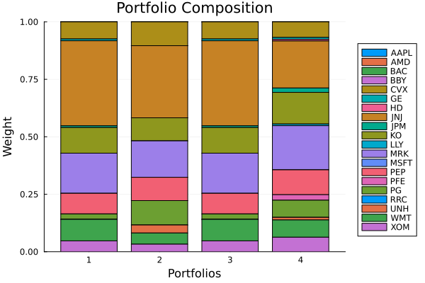
3. Cross-validation prediction
We now evaluate the benchmark and the bagged optimiser with explicit cross-validation. The cross_val_predict helper works on estimators, so we can compare the out-of-sample prediction streams directly.
Note that the optimisers we hand it carry no precomputed prior — their JuMPOptimiser has only a solver, so the prior is an estimator (the default EmpiricalPrior) refit on each training fold. This is mandatory: a precomputed prior would have been fit on the whole sample, leaking the test fold into training, so cross-validation disallows the precomputed form and requires the estimator. (See the precomputed-vs-estimator note in the MeanRisk objectives example.)
kfold = KFold(; n = 5)
cv_bench = cross_val_predict(MeanRisk(; opt = JuMPOptimiser(; slv = slv)), rd, kfold)
cv_ssr = cross_val_predict(SubsetResampling(;
                                            opt = MeanRisk(;
                                                           opt = JuMPOptimiser(; slv = slv)),
                                            subset_size = 0.7, n_subsets = 8,
                                            rng = StableRNG(123), seed = 42), rd, kfold)

scorer = NearestQuantilePrediction(; r = LowOrderMoment(; alg = SecondMoment()))
pp_bench = PopulationPredictionResult(; pred = [cv_bench])
pp_ssr = PopulationPredictionResult(; pred = [cv_ssr])
median_bench = scorer(pp_bench)
median_ssr = scorer(pp_ssr)

println("MeanRisk cross-val variance = $(expected_risk(LowOrderMoment(; alg = SecondMoment()), cv_bench))")
println("SubsetResampling cross-val variance = $(expected_risk(LowOrderMoment(; alg = SecondMoment()), cv_ssr))")

plot_cv_scores(LowOrderMoment(; alg = SecondMoment()), cv_bench)
plot_cv_scores(LowOrderMoment(; alg = SecondMoment()), cv_ssr)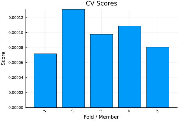
The scorer returns the prediction closest to the median of the population. On both optimisers that gives us a representative fold without hand-picking one ourselves.
println("Median benchmark fold id = $(median_bench.id)")
println("Median SSR fold id = $(median_ssr.id)")
Median benchmark fold id = nothing
Median SSR fold id = nothing4. Efficient frontier of a meta-optimiser
The frontier example from the optimiser overview used a single MeanRisk problem. Here we apply the same frontier sweep to the bagged optimiser, which gives us a frontier of bagged portfolios rather than a frontier from a single full-universe fit.
frontier_ret = ArithmeticReturn(; lb = Frontier(; N = 15))
mr_front = MeanRisk(; opt = JuMPOptimiser(; pe = pr, slv = slv, ret = frontier_ret))
ssr_front = SubsetResampling(; pe = pr,
                             opt = MeanRisk(;
                                            opt = JuMPOptimiser(; slv = slv,
                                                                ret = frontier_ret)),
                             subset_size = 0.7, n_subsets = 8, rng = StableRNG(123),
                             seed = 42)

res_mf = optimise(mr_front)
res_sf = optimise(ssr_front, rd)

rf = factory(Variance(), pr)
xs_m = [expected_risk(rf, w, pr.X) for w in res_mf.w]
ys_m = [expected_return(ArithmeticReturn(), w, pr) for w in res_mf.w]
xs_s = [expected_risk(rf, w, pr.X) for w in res_sf.w]
ys_s = [expected_return(ArithmeticReturn(), w, pr) for w in res_sf.w]

pretty_table(DataFrame(; :point => 1:length(res_mf.w),
                       :MeanRisk_max_w => [maximum(w) for w in res_mf.w],
                       :SubsetResampling_max_w => [maximum(w) for w in res_sf.w]);
             formatters = [resfmt])

plot(xs_m, ys_m; seriestype = :scatter, marker = (:circle, 5), label = "MeanRisk",
     xlabel = "Variance", ylabel = "Arithmetic return",
     title = "Frontier: plain optimiser vs bagged meta-optimiser")
plot!(xs_s, ys_s; seriestype = :scatter, marker = (:diamond, 6), label = "SubsetResampling")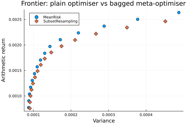
Summary
Meta-optimisers help when a single fit feels too brittle.
cross_val_predictshows how the benchmark and the bagged optimiser behave under repeated out-of-sample evaluation.SubsetResamplingsmooths allocations by averaging many subset solves.Frontier sweeps still work on the meta-optimiser, so you can compare its trade-off curve against the plain optimiser instead of choosing only one portfolio.
This page was generated using Literate.jl.