
The source files can be found in examples/.
Plotting and reporting
A portfolio is only as useful as your ability to explain it. PortfolioOptimisers.jl ships a plotting layer (loaded by bringing in StatsPlots and GraphRecipes alongside the package) that covers the whole pipeline: the inputs, the allocation, where the risk sits, realised performance, and the risk/return geometry — plus one-call dashboards that assemble several views at once. This page is a guided tour of the reporting toolkit on a single worked portfolio.
When to reach for this
Reach for these at the end of every analysis — to sanity-check inputs before optimising, to communicate an allocation, and to compare candidate strategies on the same axes. The individual plots are building blocks; the dashboards (plot_portfolio_dashboard, plot_performance_summary) are the fastest way to a complete picture.
using PortfolioOptimisers, CSV, TimeSeries, Clarabel, StatsPlots, GraphRecipes1. A worked portfolio
We build an empirical prior, a minimum-risk and a maximum-ratio book to compare, and an efficient frontier for the geometry plots.
X = TimeArray(CSV.File(joinpath(@__DIR__, "..", "SP500.csv.gz")); timestamp = :Date)[(end - 252):end]
rd = prices_to_returns(X)
pr = prior(EmpiricalPrior(), rd)

slv = Solver(; name = :clarabel, solver = Clarabel.Optimizer,
             settings = Dict("verbose" => false),
             check_sol = (; allow_local = true, allow_almost = true))
rf = 4.2 / 100 / 252

res_min = optimise(MeanRisk(; obj = MinimumRisk(),
                            opt = JuMPOptimiser(; pe = pr, slv = slv)))
res_ratio = optimise(MeanRisk(; obj = MaximumRatio(; rf = rf),
                              opt = JuMPOptimiser(; pe = pr, slv = slv)))
frontier = optimise(MeanRisk(; obj = MinimumRisk(),
                             opt = JuMPOptimiser(; pe = pr, slv = slv,
                                                 ret = ArithmeticReturn(;
                                                                        lb = Frontier(;
                                                                                      N = 15)))))
MeanRiskResult
jr ┼ JuMPOptimisationResult
│ pa ┼ ProcessedJuMPOptimiserAttributes
│ │ pr ┼ LowOrderPrior
│ │ │ X ┼ 252×20 Matrix{Float64}
│ │ │ mu ┼ 20-element Vector{Float64}
│ │ │ sigma ┼ 20×20 Matrix{Float64}
│ │ │ chol ┼ nothing
│ │ │ w ┼ nothing
│ │ │ ens ┼ nothing
│ │ │ kld ┼ nothing
│ │ │ ow ┼ nothing
│ │ │ rr ┼ nothing
│ │ │ f_mu ┼ nothing
│ │ │ f_sigma ┼ nothing
│ │ │ f_w ┴ nothing
│ │ wb ┼ WeightBounds
│ │ │ lb ┼ 20-element StepRangeLen{Float64, Base.TwicePrecision{Float64}, Base.TwicePrecision{Float64}, Int64}
│ │ │ ub ┴ 20-element StepRangeLen{Float64, Base.TwicePrecision{Float64}, Base.TwicePrecision{Float64}, Int64}
│ │ lt ┼ nothing
│ │ st ┼ nothing
│ │ lcsr ┼ nothing
│ │ ctr ┼ nothing
│ │ gcardr ┼ nothing
│ │ sgcardr ┼ nothing
│ │ smtx ┼ nothing
│ │ sgmtx ┼ nothing
│ │ slt ┼ nothing
│ │ sst ┼ nothing
│ │ sglt ┼ nothing
│ │ sgst ┼ nothing
│ │ tn ┼ nothing
│ │ fees ┼ nothing
│ │ plr ┼ nothing
│ │ ret ┼ ArithmeticReturn
│ │ │ ucs ┼ nothing
│ │ │ lb ┼ Frontier
│ │ │ │ N ┼ Int64: 15
│ │ │ │ factor ┼ Int64: 1
│ │ │ │ bound ┴ LinearBound()
│ │ │ mu ┴ 20-element Vector{Float64}
│ retcode ┼ 15-element Vector{OptimisationSuccess}
│ │ OptimisationSuccess ⋯
│ │ OptimisationSuccess ⋯
│ │ OptimisationSuccess ⋯
│ │ OptimisationSuccess ⋯
│ │ OptimisationSuccess ⋯
│ │ OptimisationSuccess ⋯
│ │ OptimisationSuccess ⋯
│ │ OptimisationSuccess ⋯
│ │ OptimisationSuccess ⋯
│ │ OptimisationSuccess ⋯
│ │ OptimisationSuccess ⋯
│ │ OptimisationSuccess ⋯
│ │ OptimisationSuccess ⋯
│ │ OptimisationSuccess ⋯
│ │ OptimisationSuccess ⋯
│ sol ┼ 15-element Vector{JuMPOptimisationSolution}
│ │ JuMPOptimisationSolution ⋯
│ │ JuMPOptimisationSolution ⋯
│ │ JuMPOptimisationSolution ⋯
│ │ JuMPOptimisationSolution ⋯
│ │ JuMPOptimisationSolution ⋯
│ │ JuMPOptimisationSolution ⋯
│ │ JuMPOptimisationSolution ⋯
│ │ JuMPOptimisationSolution ⋯
│ │ JuMPOptimisationSolution ⋯
│ │ JuMPOptimisationSolution ⋯
│ │ JuMPOptimisationSolution ⋯
│ │ JuMPOptimisationSolution ⋯
│ │ JuMPOptimisationSolution ⋯
│ │ JuMPOptimisationSolution ⋯
│ │ JuMPOptimisationSolution ⋯
│ model ┼ A JuMP Model
│ │ ├ solver: Clarabel
│ │ ├ objective_sense: MIN_SENSE
│ │ │ └ objective_function_type: QuadExpr
│ │ ├ num_variables: 22
│ │ ├ num_constraints: 6
│ │ │ ├ AffExpr in MOI.EqualTo{Float64}: 1
│ │ │ ├ AffExpr in MOI.GreaterThan{Float64}: 1
│ │ │ ├ Vector{AffExpr} in MOI.Nonnegatives: 1
│ │ │ ├ Vector{AffExpr} in MOI.Nonpositives: 1
│ │ │ ├ Vector{AffExpr} in MOI.SecondOrderCone: 1
│ │ │ └ VariableRef in MOI.Parameter{Float64}: 1
│ │ └ Names registered in the model
│ │ └ :G, :bgt, :dev_1, :dev_1_soc, :k, :lw, :obj_expr, :ret, :ret_frontier, :ret_lb, :ret_lb_var, :risk, :risk_vec, :sc, :so, :variance_flag, :variance_risk_1, :w, :w_lb, :w_ub
fb ┴ nothing2. Inspecting the inputs
Before trusting an optimisation, look at what fed it. plot_prior summarises the prior in one figure; plot_correlation and plot_mu zoom in on the covariance structure and the expected returns.
plot_prior(pr, rd)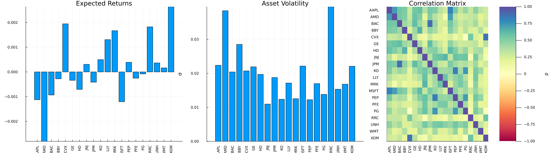
The correlation matrix on its own.
plot_correlation(pr)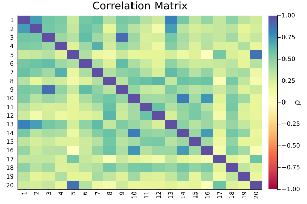
3. The allocation
plot_stacked_bar_composition puts candidate books side by side — here minimum-risk versus maximum-ratio — making the difference in concentration immediate.
plot_stacked_bar_composition([res_min, res_ratio], rd;
                             xticks = (1:2, ["Min risk", "Max ratio"]))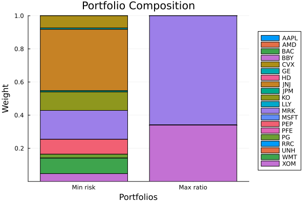
4. Where the risk sits
A book can look diversified by weight but be concentrated in risk. plot_risk_contribution decomposes the portfolio risk by asset. The risk measure comes first, and it must be configured for the data: pass factory(Variance(), pr) rather than a bare Variance() (a bare quadratic risk measure has no covariance attached yet — see the findings note). Return-based measures like ConditionalValueatRisk need no factory.
plot_risk_contribution(factory(Variance(), pr), res_min, rd)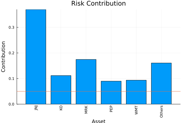
5. Realised performance
plot_ptf_cumulative_returns and plot_drawdowns show how the book would have behaved over the sample, and plot_performance_summary collects the headline performance views into one figure.
plot_ptf_cumulative_returns(res_ratio.w, rd)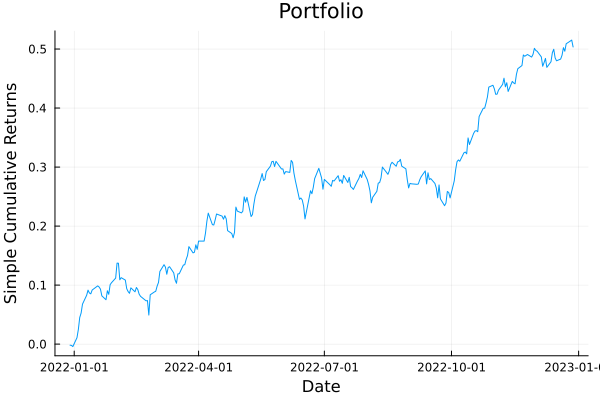
The drawdown profile.
plot_drawdowns(res_ratio.w, rd)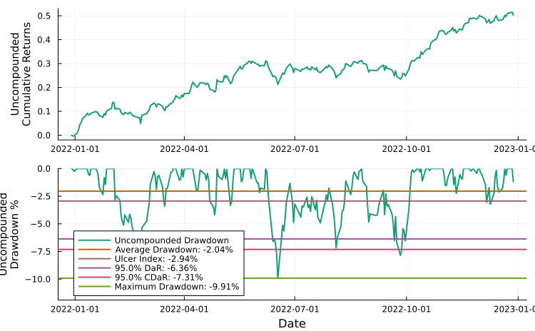
6. Risk/return geometry
plot_measures scatters portfolios on any pair of risk/return axes, and plot_efficient_frontier draws the frontier itself — the trade-off surface the optimiser traced out.
plot_efficient_frontier(frontier.w, pr; rt = frontier.ret)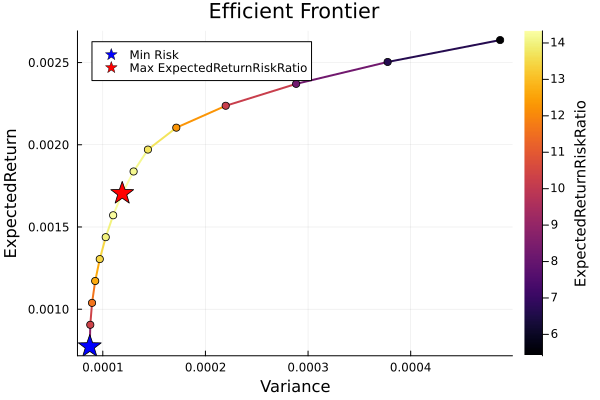
7. The dashboard
plot_portfolio_dashboard assembles composition, risk, and performance into a single report — the fastest way to a complete picture of one book.
plot_portfolio_dashboard(res_ratio, rd; r = factory(Variance(), pr))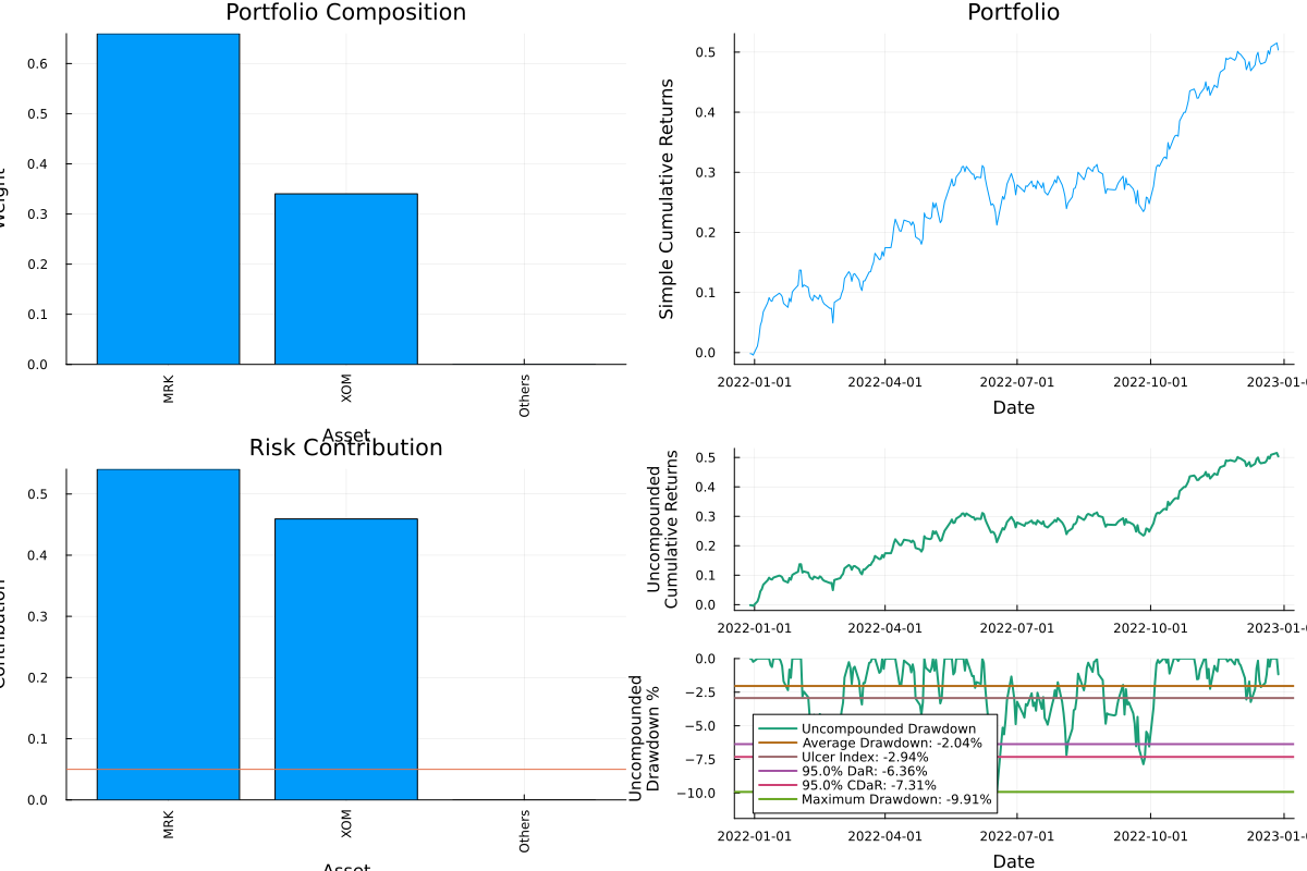
This is a selection, not the whole catalogue. The same layer also offers network and clustering views (plot_network, plot_dendrogram, plot_clusters, plot_centrality), validation plots (plot_cv_scores, plot_cv_dashboard), cost/turnover plots (plot_turnover), and higher-moment views (plot_coskewness, plot_cokurtosis) — each following the same plot_*(subject, …) convention.
This page was generated using Literate.jl.