
The source files can be found in examples/.
Specialist risk measures: BrownianDistanceVariance and VarianceSkewKurtosis
Some risk measures capture dependence structure or higher-order moment interactions that variance and CVaR miss. Two such specialist measures are:
BrownianDistanceVariance— measures non-linear dependence between portfolio returns and a reference via the Brownian (distance) covariance framework. It is zero if and only if the returns are statistically independent of the reference; variance can be zero while Brownian Distance Variance is not. It builds a T×T pairwise distance matrix so it scales quadratically in observations, not in assets.VarianceSkewKurtosis— a composite that combines variance (penalises dispersion), negative skewness (penalises asymmetry), and kurtosis (penalises heavy tails) into a single objective. It uses large PSD cones so it's best to use a solver that supports first-order algorithms such as SCS.
When to reach for this
BrownianDistanceVariance is useful when you suspect the return distribution has non-linear dependence with a factor or benchmark and want that captured in the objective. Reach for VarianceSkewKurtosis when the third and fourth moments of the portfolio return matter — e.g. when you are allocating into assets with fat tails or skewed payoffs and standard mean-variance is blind to the shape of the distribution.
Solver compatibility and dataset sizing
BrownianDistanceVariancebuilds an O(T²) distance matrix inside the model — the
number of auxiliary variables grows quadratically with observations. This example uses a 50-observation slice to keep the model small.
VarianceSkewKurtosisrequires SCS (or another solver that handles polynomial PSD
cones). It will fail silently or produce wrong results with a continuous-only solver like Clarabel. The high-order prior (HighOrderPriorEstimator) must also be used, as it pre-computes the coskewness and cokurtosis tensors the risk measure needs. This example also uses a 50-observation slice for the same reason.
using PortfolioOptimisers, PrettyTables, DataFrames

resfmt = (v, i, j) -> begin
    if j == 1
        return v
    else
        return isa(v, Number) ? "$(round(v * 100, digits = 3)) %" : v
    end
end;

using CSV, TimeSeries, Clarabel, SCS
1. Shared data — 50-observation slice
Both measures in this example use the same short 50-observation slice. BrownianDistanceVariance builds an O(T²) distance matrix, so T is the binding constraint on model size. VarianceSkewKurtosis needs a HighOrderPriorEstimator whose coskewness/cokurtosis computation also scales with T.
X = TimeArray(CSV.File(joinpath(@__DIR__, "..", "SP500.csv.gz")); timestamp = :Date)[(end - 50):end]
rd = prices_to_returns(X)
pr = prior(EmpiricalPrior(), rd)

slv = [Solver(; name = :clarabel1, solver = Clarabel.Optimizer,
              settings = Dict("verbose" => false),
              check_sol = (; allow_local = true, allow_almost = true)),
       Solver(; name = :clarabel2, solver = Clarabel.Optimizer,
              settings = Dict("verbose" => false, "max_step_fraction" => 0.95),
              check_sol = (; allow_local = true, allow_almost = true)),
       Solver(; name = :clarabel3, solver = Clarabel.Optimizer,
              settings = Dict("verbose" => false, "max_step_fraction" => 0.9),
              check_sol = (; allow_local = true, allow_almost = true)),
       Solver(; name = :clarabel4, solver = Clarabel.Optimizer,
              settings = Dict("verbose" => false, "max_step_fraction" => 0.85),
              check_sol = (; allow_local = true, allow_almost = true))]

opt = JuMPOptimiser(; pe = pr, slv = slv)
JuMPOptimiser
pe ┼ LowOrderPrior
│ X ┼ 50×20 Matrix{Float64}
│ mu ┼ 20-element Vector{Float64}
│ sigma ┼ 20×20 Matrix{Float64}
│ chol ┼ nothing
│ w ┼ nothing
│ ens ┼ nothing
│ kld ┼ nothing
│ ow ┼ nothing
│ rr ┼ nothing
│ f_mu ┼ nothing
│ f_sigma ┼ nothing
│ f_w ┴ nothing
slv ┼ 4-element Vector{Solver}
│ Solver ⋯
│ Solver ⋯
│ Solver ⋯
│ Solver ⋯
wb ┼ WeightBounds
│ lb ┼ Float64: 0.0
│ ub ┴ Float64: 1.0
bgt ┼ Float64: 1.0
sbgt ┼ nothing
lt ┼ nothing
st ┼ nothing
lcse ┼ nothing
cte ┼ nothing
gcarde ┼ nothing
sgcarde ┼ nothing
smtx ┼ nothing
sgmtx ┼ nothing
slt ┼ nothing
sst ┼ nothing
sglt ┼ nothing
sgst ┼ nothing
tn ┼ nothing
fees ┼ nothing
sets ┼ nothing
tr ┼ nothing
ple ┼ nothing
ret ┼ ArithmeticReturn
│ ucs ┼ nothing
│ lb ┼ nothing
│ mu ┴ nothing
sca ┼ SumScalariser()
ccnt ┼ nothing
cobj ┼ nothing
sc ┼ Int64: 1
so ┼ Int64: 1
ss ┼ nothing
card ┼ nothing
scard ┼ nothing
wn2 ┼ nothing
wnp ┼ nothing
wninf ┼ nothing
l1 ┼ nothing
l2 ┼ nothing
linf ┼ nothing
lp ┼ nothing
brt ┼ Bool: false
cle_pr ┼ Bool: true
strict ┴ Bool: false2. Brownian Distance Variance
### 2.1 Default formulationBrownianDistanceVariance uses a Norm-1 cone constraint by default (NormOneConeBrownianDistanceVariance). The T×T distance matrix is linearised via auxiliary variables so Clarabel can handle it as a conic programme.
res_bdvar = optimise(MeanRisk(; r = BrownianDistanceVariance(), opt = opt))MeanRiskResult
jr ┼ JuMPOptimisationResult
│ pa ┼ ProcessedJuMPOptimiserAttributes
│ │ pr ┼ LowOrderPrior
│ │ │ X ┼ 50×20 Matrix{Float64}
│ │ │ mu ┼ 20-element Vector{Float64}
│ │ │ sigma ┼ 20×20 Matrix{Float64}
│ │ │ chol ┼ nothing
│ │ │ w ┼ nothing
│ │ │ ens ┼ nothing
│ │ │ kld ┼ nothing
│ │ │ ow ┼ nothing
│ │ │ rr ┼ nothing
│ │ │ f_mu ┼ nothing
│ │ │ f_sigma ┼ nothing
│ │ │ f_w ┴ nothing
│ │ wb ┼ WeightBounds
│ │ │ lb ┼ 20-element StepRangeLen{Float64, Base.TwicePrecision{Float64}, Base.TwicePrecision{Float64}, Int64}
│ │ │ ub ┴ 20-element StepRangeLen{Float64, Base.TwicePrecision{Float64}, Base.TwicePrecision{Float64}, Int64}
│ │ lt ┼ nothing
│ │ st ┼ nothing
│ │ lcsr ┼ nothing
│ │ ctr ┼ nothing
│ │ gcardr ┼ nothing
│ │ sgcardr ┼ nothing
│ │ smtx ┼ nothing
│ │ sgmtx ┼ nothing
│ │ slt ┼ nothing
│ │ sst ┼ nothing
│ │ sglt ┼ nothing
│ │ sgst ┼ nothing
│ │ tn ┼ nothing
│ │ fees ┼ nothing
│ │ plr ┼ nothing
│ │ ret ┼ ArithmeticReturn
│ │ │ ucs ┼ nothing
│ │ │ lb ┼ nothing
│ │ │ mu ┴ 20-element Vector{Float64}
│ retcode ┼ OptimisationSuccess
│ │ res ┴ Dict{Any, Any}: Dict{Any, Any}()
│ sol ┼ JuMPOptimisationSolution
│ │ w ┴ 20-element Vector{Float64}
│ model ┼ A JuMP Model
│ │ ├ solver: Clarabel
│ │ ├ objective_sense: MIN_SENSE
│ │ │ └ objective_function_type: QuadExpr
│ │ ├ num_variables: 1295
│ │ ├ num_constraints: 1278
│ │ │ ├ AffExpr in MOI.EqualTo{Float64}: 1
│ │ │ ├ Vector{AffExpr} in MOI.Nonnegatives: 1
│ │ │ ├ Vector{AffExpr} in MOI.Nonpositives: 1
│ │ │ └ Vector{AffExpr} in MOI.NormOneCone: 1275
│ │ └ Names registered in the model
│ │ └ :Dt, :Dx, :X, :bdvariance_risk, :bgt, :cbdvariance_noc, :k, :lw, :net_X, :obj_expr, :ret, :risk, :risk_vec, :sc, :so, :w, :w_lb, :w_ub
fb ┴ nothingAn alternative formulation (IneqBrownianDistanceVariance) uses inequality constraints rather than a cone. On small problems the results are equivalent; on larger problems the inequality form may be faster because it avoids a large cone.
res_bdvar_ineq = optimise(MeanRisk(;
                                   r = BrownianDistanceVariance(;
                                                                alg2 = IneqBrownianDistanceVariance()),
                                   opt = opt))
MeanRiskResult
jr ┼ JuMPOptimisationResult
│ pa ┼ ProcessedJuMPOptimiserAttributes
│ │ pr ┼ LowOrderPrior
│ │ │ X ┼ 50×20 Matrix{Float64}
│ │ │ mu ┼ 20-element Vector{Float64}
│ │ │ sigma ┼ 20×20 Matrix{Float64}
│ │ │ chol ┼ nothing
│ │ │ w ┼ nothing
│ │ │ ens ┼ nothing
│ │ │ kld ┼ nothing
│ │ │ ow ┼ nothing
│ │ │ rr ┼ nothing
│ │ │ f_mu ┼ nothing
│ │ │ f_sigma ┼ nothing
│ │ │ f_w ┴ nothing
│ │ wb ┼ WeightBounds
│ │ │ lb ┼ 20-element StepRangeLen{Float64, Base.TwicePrecision{Float64}, Base.TwicePrecision{Float64}, Int64}
│ │ │ ub ┴ 20-element StepRangeLen{Float64, Base.TwicePrecision{Float64}, Base.TwicePrecision{Float64}, Int64}
│ │ lt ┼ nothing
│ │ st ┼ nothing
│ │ lcsr ┼ nothing
│ │ ctr ┼ nothing
│ │ gcardr ┼ nothing
│ │ sgcardr ┼ nothing
│ │ smtx ┼ nothing
│ │ sgmtx ┼ nothing
│ │ slt ┼ nothing
│ │ sst ┼ nothing
│ │ sglt ┼ nothing
│ │ sgst ┼ nothing
│ │ tn ┼ nothing
│ │ fees ┼ nothing
│ │ plr ┼ nothing
│ │ ret ┼ ArithmeticReturn
│ │ │ ucs ┼ nothing
│ │ │ lb ┼ nothing
│ │ │ mu ┴ 20-element Vector{Float64}
│ retcode ┼ OptimisationSuccess
│ │ res ┴ Dict{Any, Any}: Dict{Any, Any}()
│ sol ┼ JuMPOptimisationSolution
│ │ w ┴ 20-element Vector{Float64}
│ model ┼ A JuMP Model
│ │ ├ solver: Clarabel
│ │ ├ objective_sense: MIN_SENSE
│ │ │ └ objective_function_type: QuadExpr
│ │ ├ num_variables: 1295
│ │ ├ num_constraints: 5
│ │ │ ├ AffExpr in MOI.EqualTo{Float64}: 1
│ │ │ ├ Vector{AffExpr} in MOI.Nonnegatives: 3
│ │ │ └ Vector{AffExpr} in MOI.Nonpositives: 1
│ │ └ Names registered in the model
│ │ └ :Dt, :Dx, :X, :bdvariance_risk, :bgt, :cn_bdvariance, :cp_bdvariance, :k, :lw, :net_X, :obj_expr, :ret, :risk, :risk_vec, :sc, :so, :w, :w_lb, :w_ub
fb ┴ nothing2.2 Alternative formulations
A second formulation switch controls the rank constraint used for the distance matrix: QuadRiskExpr (default) or RSOCRiskExpr. The latter uses a rotated second-order cone and can be faster for very dense problems.
res_bdvar_rsoc = optimise(MeanRisk(; r = BrownianDistanceVariance(; alg1 = RSOCRiskExpr()),
                                   opt = opt))

pretty_table(DataFrame(; :assets => rd.nx, :BDVar_default => res_bdvar.w,
                       :BDVar_ineq => res_bdvar_ineq.w, :BDVar_rsoc => res_bdvar_rsoc.w);
             formatters = [resfmt])
┌────────┬───────────────┬────────────┬────────────┐
│ assets │ BDVar_default │ BDVar_ineq │ BDVar_rsoc │
│ String │ Float64 │ Float64 │ Float64 │
├────────┼───────────────┼────────────┼────────────┤
│ AAPL │ 0.0 % │ 0.0 % │ -0.0 % │
│ AMD │ 0.0 % │ 0.0 % │ -0.0 % │
│ BAC │ 0.0 % │ 0.0 % │ -0.0 % │
│ BBY │ 0.0 % │ 0.0 % │ -0.0 % │
│ CVX │ 6.687 % │ 6.687 % │ 6.687 % │
│ GE │ 0.0 % │ 0.0 % │ -0.0 % │
│ HD │ 0.0 % │ 0.0 % │ -0.0 % │
│ JNJ │ 43.573 % │ 43.573 % │ 43.586 % │
│ JPM │ 0.0 % │ 0.0 % │ -0.0 % │
│ KO │ 0.0 % │ 0.0 % │ -0.0 % │
│ LLY │ 0.0 % │ 0.0 % │ -0.0 % │
│ MRK │ 4.505 % │ 4.506 % │ 4.498 % │
│ MSFT │ 0.0 % │ 0.0 % │ -0.0 % │
│ PEP │ 6.377 % │ 6.377 % │ 6.379 % │
│ PFE │ 0.0 % │ 0.0 % │ -0.0 % │
│ ⋮ │ ⋮ │ ⋮ │ ⋮ │
└────────┴───────────────┴────────────┴────────────┘
5 rows omittedThe three formulations produce the same portfolio — the differences are only in how the conic model is assembled, not in what it optimises.
The composition plot shows that Brownian Distance Variance concentrates into a different set of names than plain variance minimisation, reflecting its sensitivity to non-linear dependence rather than just squared-deviation spread.
res_var = optimise(MeanRisk(; r = Variance(), opt = opt))

using StatsPlots, GraphRecipes
plot_stacked_bar_composition([res_var, res_bdvar], rd)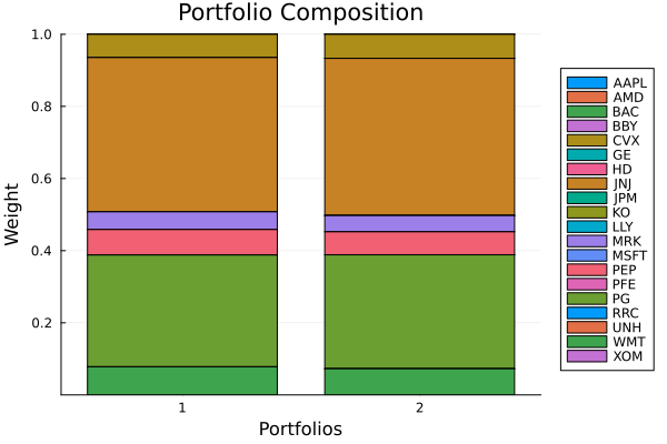
3. VarianceSkewKurtosis
3.1 High-order prior and SCS solver
VarianceSkewKurtosis requires SCS and a HighOrderPriorEstimator prior. We reuse the same 50-observation slice already loaded in section 1.
pr_ho = prior(HighOrderPriorEstimator(), rd)

scs_slv = Solver(; name = :scs, solver = SCS.Optimizer, settings = "verbose" => false,
                 check_sol = (; allow_local = true, allow_almost = true))
opt_ho = JuMPOptimiser(; pe = pr_ho, slv = scs_slv)
JuMPOptimiser
pe ┼ HighOrderPrior
│ pr ┼ LowOrderPrior
│ │ X ┼ 50×20 Matrix{Float64}
│ │ mu ┼ 20-element Vector{Float64}
│ │ sigma ┼ 20×20 Matrix{Float64}
│ │ chol ┼ nothing
│ │ w ┼ nothing
│ │ ens ┼ nothing
│ │ kld ┼ nothing
│ │ ow ┼ nothing
│ │ rr ┼ nothing
│ │ f_mu ┼ nothing
│ │ f_sigma ┼ nothing
│ │ f_w ┴ nothing
│ kt ┼ 400×400 Matrix{Float64}
│ D2 ┼ 400×210 SparseArrays.SparseMatrixCSC{Int64, Int64}
│ L2 ┼ 210×400 SparseArrays.SparseMatrixCSC{Int64, Int64}
│ S2 ┼ 210×400 SparseArrays.SparseMatrixCSC{Int64, Int64}
│ sk ┼ 20×400 Matrix{Float64}
│ V ┼ 20×20 Matrix{Float64}
│ skmp ┼ MatrixProcessing
│ │ pdm ┼ Posdef
│ │ │ alg ┼ UnionAll: NearestCorrelationMatrix.Newton
│ │ │ kwargs ┴ @NamedTuple{}: NamedTuple()
│ │ dn ┼ nothing
│ │ dt ┼ nothing
│ │ alg ┼ nothing
│ │ order ┴ NTuple{4, Symbol}: (:pdm, :dn, :dt, :alg)
│ f_kt ┼ nothing
│ f_sk ┼ nothing
│ f_V ┴ nothing
slv ┼ Solver
│ name ┼ Symbol: :scs
│ solver ┼ DataType: DataType
│ settings ┼ Pair{String, Bool}: "verbose" => false
│ check_sol ┼ @NamedTuple{allow_local::Bool, allow_almost::Bool}: (allow_local = true, allow_almost = true)
│ add_bridges ┴ Bool: true
wb ┼ WeightBounds
│ lb ┼ Float64: 0.0
│ ub ┴ Float64: 1.0
bgt ┼ Float64: 1.0
sbgt ┼ nothing
lt ┼ nothing
st ┼ nothing
lcse ┼ nothing
cte ┼ nothing
gcarde ┼ nothing
sgcarde ┼ nothing
smtx ┼ nothing
sgmtx ┼ nothing
slt ┼ nothing
sst ┼ nothing
sglt ┼ nothing
sgst ┼ nothing
tn ┼ nothing
fees ┼ nothing
sets ┼ nothing
tr ┼ nothing
ple ┼ nothing
ret ┼ ArithmeticReturn
│ ucs ┼ nothing
│ lb ┼ nothing
│ mu ┴ nothing
sca ┼ SumScalariser()
ccnt ┼ nothing
cobj ┼ nothing
sc ┼ Int64: 1
so ┼ Int64: 1
ss ┼ nothing
card ┼ nothing
scard ┼ nothing
wn2 ┼ nothing
wnp ┼ nothing
wninf ┼ nothing
l1 ┼ nothing
l2 ┼ nothing
linf ┼ nothing
lp ┼ nothing
brt ┼ Bool: false
cle_pr ┼ Bool: true
strict ┴ Bool: false3.2 Default composite
VarianceSkewKurtosis combines three sub-measures:
Variance— penalises dispersion.Skewness(negative skewness convention) — penalises left-skewed returns.Kurtosis— penalises fat tails.
The default scales are 1:1:1. Scaling one component higher makes the objective more sensitive to that moment.
res_vsk = optimise(MeanRisk(; r = VarianceSkewKurtosis(), opt = opt_ho), rd)
println("VarianceSkewKurtosis retcode: $(res_vsk.retcode)")
VarianceSkewKurtosis retcode: OptimisationSuccess
res ┴ Dict{Any, Any}: Dict{Any, Any}()3.3 Custom component scales
Passing custom Skewness and Kurtosis with scaled settings (MaxRiskMeasureSettings for skewness and RiskMeasureSettings for kurtosis) lets you control how much each higher-moment penalty contributes relative to variance.
r_vsk_heavy = VarianceSkewKurtosis(;
                                   sk = Skewness(;
                                                 settings = MaxRiskMeasureSettings(;
                                                                                   scale = 2.0)),
                                   kt = Kurtosis(;
                                                 settings = RiskMeasureSettings(;
                                                                                scale = 2.0)))
res_vsk_heavy = optimise(MeanRisk(; r = r_vsk_heavy, opt = opt_ho), rd)
MeanRiskResult
jr ┼ JuMPOptimisationResult
│ pa ┼ ProcessedJuMPOptimiserAttributes
│ │ pr ┼ HighOrderPrior
│ │ │ pr ┼ LowOrderPrior
│ │ │ │ X ┼ 50×20 Matrix{Float64}
│ │ │ │ mu ┼ 20-element Vector{Float64}
│ │ │ │ sigma ┼ 20×20 Matrix{Float64}
│ │ │ │ chol ┼ nothing
│ │ │ │ w ┼ nothing
│ │ │ │ ens ┼ nothing
│ │ │ │ kld ┼ nothing
│ │ │ │ ow ┼ nothing
│ │ │ │ rr ┼ nothing
│ │ │ │ f_mu ┼ nothing
│ │ │ │ f_sigma ┼ nothing
│ │ │ │ f_w ┴ nothing
│ │ │ kt ┼ 400×400 Matrix{Float64}
│ │ │ D2 ┼ 400×210 SparseArrays.SparseMatrixCSC{Int64, Int64}
│ │ │ L2 ┼ 210×400 SparseArrays.SparseMatrixCSC{Int64, Int64}
│ │ │ S2 ┼ 210×400 SparseArrays.SparseMatrixCSC{Int64, Int64}
│ │ │ sk ┼ 20×400 Matrix{Float64}
│ │ │ V ┼ 20×20 Matrix{Float64}
│ │ │ skmp ┼ MatrixProcessing
│ │ │ │ pdm ┼ Posdef
│ │ │ │ │ alg ┼ UnionAll: NearestCorrelationMatrix.Newton
│ │ │ │ │ kwargs ┴ @NamedTuple{}: NamedTuple()
│ │ │ │ dn ┼ nothing
│ │ │ │ dt ┼ nothing
│ │ │ │ alg ┼ nothing
│ │ │ │ order ┴ NTuple{4, Symbol}: (:pdm, :dn, :dt, :alg)
│ │ │ f_kt ┼ nothing
│ │ │ f_sk ┼ nothing
│ │ │ f_V ┴ nothing
│ │ wb ┼ WeightBounds
│ │ │ lb ┼ 20-element StepRangeLen{Float64, Base.TwicePrecision{Float64}, Base.TwicePrecision{Float64}, Int64}
│ │ │ ub ┴ 20-element StepRangeLen{Float64, Base.TwicePrecision{Float64}, Base.TwicePrecision{Float64}, Int64}
│ │ lt ┼ nothing
│ │ st ┼ nothing
│ │ lcsr ┼ nothing
│ │ ctr ┼ nothing
│ │ gcardr ┼ nothing
│ │ sgcardr ┼ nothing
│ │ smtx ┼ nothing
│ │ sgmtx ┼ nothing
│ │ slt ┼ nothing
│ │ sst ┼ nothing
│ │ sglt ┼ nothing
│ │ sgst ┼ nothing
│ │ tn ┼ nothing
│ │ fees ┼ nothing
│ │ plr ┼ nothing
│ │ ret ┼ ArithmeticReturn
│ │ │ ucs ┼ nothing
│ │ │ lb ┼ nothing
│ │ │ mu ┴ 20-element Vector{Float64}
│ retcode ┼ OptimisationSuccess
│ │ res ┴ Dict{Any, Any}: Dict{Any, Any}()
│ sol ┼ JuMPOptimisationSolution
│ │ w ┴ 20-element Vector{Float64}
│ model ┼ A JuMP Model
│ │ ├ solver: SCS
│ │ ├ objective_sense: MIN_SENSE
│ │ │ └ objective_function_type: AffExpr
│ │ ├ num_variables: 26585
│ │ ├ num_constraints: 4
│ │ │ ├ AffExpr in MOI.EqualTo{Float64}: 1
│ │ │ ├ Vector{AffExpr} in MOI.Nonnegatives: 1
│ │ │ ├ Vector{AffExpr} in MOI.Nonpositives: 1
│ │ │ └ Vector{AffExpr} in MOI.PositiveSemidefiniteConeSquare: 1
│ │ └ Names registered in the model
│ │ └ :L2W1_vr_sk_kt, :M_vr_sk_kt, :M_vr_sk_kt_PSD, :W1_vr_sk_kt, :W2_vr_sk_kt, :W3_vr_sk_kt, :bgt, :k, :kt_risk_1, :lw, :obj_expr, :ret, :risk, :risk_vec, :sc, :sk_risk_1, :so, :vr_risk_1, :vr_sk_kt_risk_1, :w, :w_lb, :w_ub
fb ┴ nothingCompare the two allocations. Heavier skewness/kurtosis penalties push the optimiser further away from fat-tailed or left-skewed names.
pretty_table(DataFrame(; :assets => rd.nx, :VarianceSkewKurtosis => res_vsk.w,
                       :VSK_heavy_tail => res_vsk_heavy.w); formatters = [resfmt])
┌────────┬──────────────────────┬────────────────┐
│ assets │ VarianceSkewKurtosis │ VSK_heavy_tail │
│ String │ Float64 │ Float64 │
├────────┼──────────────────────┼────────────────┤
│ AAPL │ 0.004 % │ 0.011 % │
│ AMD │ 0.005 % │ 0.0 % │
│ BAC │ 4.666 % │ 4.692 % │
│ BBY │ 0.765 % │ 0.794 % │
│ CVX │ 5.839 % │ 5.781 % │
│ GE │ 3.994 % │ 3.984 % │
│ HD │ 1.795 % │ 1.857 % │
│ JNJ │ 8.999 % │ 8.984 % │
│ JPM │ 5.485 % │ 5.509 % │
│ KO │ 6.648 % │ 6.649 % │
│ LLY │ 7.755 % │ 7.764 % │
│ MRK │ 9.094 % │ 9.064 % │
│ MSFT │ 0.755 % │ 0.831 % │
│ PEP │ 8.311 % │ 8.288 % │
│ PFE │ 6.668 % │ 6.661 % │
│ ⋮ │ ⋮ │ ⋮ │
└────────┴──────────────────────┴────────────────┘
5 rows omitted3.4 Comparison with plain variance (SCS)
We compare the VSK portfolio against a plain minimum-variance portfolio solved with SCS on the same 50-observation prior, so the only difference is the risk measure.
res_var_scs = optimise(MeanRisk(; r = Variance(), opt = opt_ho))

plot_stacked_bar_composition([res_var_scs, res_vsk, res_vsk_heavy], rd)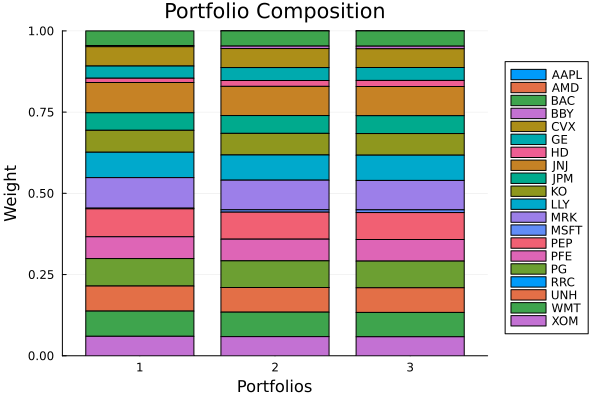
Summary
BrownianDistanceVarianceuses a 50-observation slice with Clarabel. It captures non-linear dependence via a quadratic T×T distance matrix; keep T small (the O(T²) model size is the limiting factor, not the number of assets).VarianceSkewKurtosismust use SCS (polynomial PSD cones). Pair it withHighOrderPriorEstimatorand a short observation window to keep the higher-moment tensor computation feasible.
This page was generated using Literate.jl.