PortfolioOptimisers.jl
Portfolio optimisation library for Julia
Democratising, demystifying, and derisking investing

Priors and views
Empirical, factor, and high-order priors. Impose views with the Black-Litterman family, entropy pooling, or opinion pooling. Swapping the prior leaves the optimiser untouched.
Robust moment estimation
Gerber, Gerber-IQ, and Smyth-Broby covariances, mutual information and distance covariance, denoising, detoning, regime adjustment, coskewness, and cokurtosis.
Over 50 risk measures
Variance, semi-moments, mean absolute deviation, VaR, CVaR, EVaR, RLVaR, drawdowns, ordered weights arrays, and tail ranges. Combine several in one objective, and/or use them as a limit.
An optimiser for every mandate
Mean-risk, risk budgeting, near-optimal centering, hierarchical risk parity, HERC, Schur complement, naïve, and the meta-optimisers that nest, stack, and resample them.
Constraints and costs
Budget, group, factor exposure, cardinality, turnover, tracking, phylogeny, and centrality constraints, plus fees and market impact. Add your own JuMP expressions.
Validation and tuning
Walk-forward and combinatorial cross-validation, grid and randomised hyperparameter search, pipelines, and time-dependent constraints.
Welcome to PortfolioOptimisers.jl
PortfolioOptimisers.jl is a portfolio optimisation (portfolio optimization) library for Julia. Every component is an immutable estimator you compose, so a prior, a risk measure or a constraint swaps out without touching the optimiser.
Investing conveys real risk, the entire point of portfolio optimisation is to minimise it to tolerable levels. The examples use outdated data and a variety of stocks (including what I consider to be meme stocks) for demonstration purposes only. None of the information in this documentation should be taken as financial advice. Any advice is limited to improving portfolio construction, most of which is common investment and statistical knowledge.
Caveat emptor
PortfolioOptimisers.jlis under active development and still inv0.*.*. Therefore, breaking changes should be expected withv0.X.0releases. All other releases will fall underv0.X.Y.- The documentation is still under construction.
- Testing coverage is still under
95 %. We're mainly missing assertion tests, but some lesser used features are partially or wholly untested. - Please feel free to submit issues, discussions and/or PRs regarding missing docs, examples, features, tests, and bugs.
Installation
PortfolioOptimisers.jl is a registered package, so installation is as simple as:
julia> using Pkgjulia> Pkg.add(PackageSpec(; name = "PortfolioOptimisers"))Roadmap
The Issues page is used as a tracker for bugs, feature requests, plans, and works in progress.
The dev branch is used as a staging ground before merging into
main.
Quick-start
The library is quite powerful and extremely flexible. Here is what a very basic end-to-end workflow can look like. The examples contain more thorough explanations and demos. The API docs contain toy examples of the many, many features.
First we import the packages we will need for the example.
StatsPlotsandGraphRecipesare needed to load the plotting extension.ClarabelandHiGHSare the optimisers we will use.CSV,TimeSeriesandDataFramesfor loading and preprocessing price data.PrettyTablesfor displaying the results.
# Import module and plotting extension.using PortfolioOptimisers, StatsPlots, GraphRecipes# Import optimisers.using Clarabel, HiGHS# Load and preprocess data.using CSV, TimeSeries, DataFrames# Pretty printing.using PrettyTables# Format for pretty tables.fmt1 = (v, i, j) -> begin if j == 1 return Date(v) else return v endend;fmt2 = (v, i, j) -> begin if j ∈ (1, 2, 3) return v else return isa(v, Number) ? "$(round(v*100, digits=3)) %" : v endend;We will use the S&P 500 sample dataset that ships with the documentation: daily adjusted close prices for 20 large-cap stocks. To keep the example quick, we use the most recent year (253 observations).
# Load the shipped S&P 500 price data as a TimeArray.prices = TimeArray(CSV.File(joinpath(@__DIR__, "examples", "SP500.csv.gz")); timestamp = :Date)[(end - 252):end]pretty_table(prices[(end - 5):end]; formatters = [fmt1])┌────────────┬─────────┬─────────┬─────────┬─────────┬─────────┬─────────┬─────────┬─────────┬─────────┬─────────┬─────────┬─────────┬─────────┬─────────┬─────────┬─────────┬─────────┬─────────┬─────────┬─────────┐
│ timestamp │ AAPL │ AMD │ BAC │ BBY │ CVX │ GE │ HD │ JNJ │ JPM │ KO │ LLY │ MRK │ MSFT │ PEP │ PFE │ PG │ RRC │ UNH │ WMT │ XOM │
│ Date │ Float64 │ Float64 │ Float64 │ Float64 │ Float64 │ Float64 │ Float64 │ Float64 │ Float64 │ Float64 │ Float64 │ Float64 │ Float64 │ Float64 │ Float64 │ Float64 │ Float64 │ Float64 │ Float64 │ Float64 │
├────────────┼─────────┼─────────┼─────────┼─────────┼─────────┼─────────┼─────────┼─────────┼─────────┼─────────┼─────────┼─────────┼─────────┼─────────┼─────────┼─────────┼─────────┼─────────┼─────────┼─────────┤
│ 2022-12-20 │ 131.916 │ 65.05 │ 31.729 │ 77.371 │ 169.497 │ 62.604 │ 310.342 │ 173.109 │ 127.844 │ 61.841 │ 357.55 │ 108.229 │ 240.67 │ 178.765 │ 49.754 │ 147.661 │ 25.65 │ 516.245 │ 142.919 │ 104.964 │
│ 2022-12-21 │ 135.057 │ 67.68 │ 32.212 │ 78.729 │ 171.49 │ 64.67 │ 314.798 │ 175.09 │ 129.282 │ 62.836 │ 365.872 │ 109.611 │ 243.287 │ 180.017 │ 50.084 │ 149.015 │ 26.574 │ 523.519 │ 144.04 │ 106.312 │
│ 2022-12-22 │ 131.846 │ 63.86 │ 31.927 │ 78.563 │ 168.918 │ 63.727 │ 311.604 │ 174.45 │ 127.814 │ 62.383 │ 363.187 │ 109.739 │ 237.077 │ 178.627 │ 50.065 │ 149.359 │ 25.232 │ 523.072 │ 142.354 │ 104.168 │
│ 2022-12-23 │ 131.477 │ 64.52 │ 32.005 │ 79.432 │ 174.14 │ 63.742 │ 314.177 │ 174.893 │ 128.421 │ 62.855 │ 365.762 │ 110.35 │ 237.614 │ 179.781 │ 50.249 │ 149.781 │ 26.226 │ 527.26 │ 142.641 │ 106.922 │
│ 2022-12-27 │ 129.652 │ 63.27 │ 32.065 │ 79.93 │ 176.329 │ 64.561 │ 314.985 │ 174.844 │ 128.871 │ 63.24 │ 362.76 │ 110.607 │ 235.852 │ 180.58 │ 49.57 │ 151.086 │ 26.375 │ 527.935 │ 142.681 │ 108.408 │
│ 2022-12-28 │ 125.674 │ 62.57 │ 32.301 │ 78.279 │ 173.728 │ 63.883 │ 311.22 │ 174.085 │ 129.575 │ 62.609 │ 363.098 │ 109.581 │ 233.434 │ 179.278 │ 49.25 │ 149.133 │ 24.497 │ 524.422 │ 140.181 │ 106.627 │
└────────────┴─────────┴─────────┴─────────┴─────────┴─────────┴─────────┴─────────┴─────────┴─────────┴─────────┴─────────┴─────────┴─────────┴─────────┴─────────┴─────────┴─────────┴─────────┴─────────┴─────────┘The dataset above is a plain (gzipped) CSV with a Date column and one column per asset, so any price history in that shape will do. To pull live data instead, you can download it with YFinance.jl and assemble a TimeArray:
using YFinance, TimeSeries# Convert a YFinance price dictionary into a TimeArray.function stock_price_to_time_array(x) # Only get the keys that are not ticker or datetime. coln = collect(keys(x))[3:end] # Convert the dictionary into a matrix. m = hcat([x[k] for k in coln]...) return TimeArray(x["timestamp"], m, Symbol.(coln), x["ticker"])endassets = sort!(["AAPL", "AMD", "BAC", "BBY", "CVX", "GE", "HD", "JNJ", "JPM", "KO", "LLY", "MRK", "MSFT", "PEP", "PFE", "PG", "RRC", "UNH", "WMT", "XOM"])# Download the adjusted close prices and assemble a single TimeArray.prices = get_prices.(assets; startdt = "2024-01-01", enddt = "2025-01-01")prices = stock_price_to_time_array.(prices)prices = hcat(prices...)cidx = colnames(prices)[occursin.(r"adj", string.(colnames(prices)))]prices = prices[cidx]TimeSeries.rename!(prices, Symbol.(assets))Now we can compute our returns by calling prices_to_returns.
# Compute the returns.rd = prices_to_returns(prices)ReturnsResult
nx ┼ 20-element Vector{String}
X ┼ 252×20 Matrix{Float64}
nf ┼ nothing
F ┼ nothing
nb ┼ nothing
B ┼ nothing
ts ┼ 252-element Vector{Date}
iv ┼ nothing
ivpa ┼ nothing
pnl ┼ AssetPanel
│ pf ┼ Vector{AbstractPanelField}: AbstractPanelField[]
│ amsk ┼ 252×20 AllTrueMask
│ emsk ┴ 252×20 AllTrueMask
PortfolioOptimisers.jl uses JuMP for handling the optimisation problems, which means it is solver agnostic and therefore does not ship with any pre-installed solver. Solver lets us define the optimiser factory, its solver-specific settings, and JuMP's solution acceptance criteria.
# Define the continuous solver.slv = Solver(; name = :clarabel1, solver = Clarabel.Optimizer, settings = Dict("verbose" => false, "max_step_fraction" => 0.9), check_sol = (; allow_local = true, allow_almost = true))Solver
name ┼ Symbol: :clarabel1
solver ┼ UnionAll: Clarabel.MOIwrapper.Optimizer
settings ┼ Dict{String, Real}: Dict{String, Real}("max_step_fraction" => 0.9, "verbose" => false)
check_sol ┼ @NamedTuple{allow_local::Bool, allow_almost::Bool}: (allow_local = true, allow_almost = true)
add_bridges ┴ Bool: true
PortfolioOptimisers.jl implements a number of optimisation types as estimators. All the ones which use mathematical optimisation require a JuMPOptimiser structure which defines general solver constraints. This structure in turn requires an instance (or vector) of Solver.
opt = JuMPOptimiser(; slv = slv);Here we will use the traditional Mean-Risk MeanRisk optimisation estimator, which defaults to the Markowitz optimisation (minimum risk mean-variance optimisation).
# Vanilla (Markowitz) mean risk optimisation.mr = MeanRisk(; opt = opt)MeanRisk
opt ┼ JuMPOptimiser
│ pe ┼ EmpiricalPrior
│ │ ce ┼ PortfolioOptimisersCovariance
│ │ │ ce ┼ Covariance
│ │ │ │ me ┼ SimpleExpectedReturns
│ │ │ │ │ w ┴ nothing
│ │ │ │ ce ┼ GeneralCovariance
│ │ │ │ │ ce ┼ SimpleCovariance: SimpleCovariance(true)
│ │ │ │ │ w ┴ nothing
│ │ │ │ alg ┼ FullMoment()
│ │ │ │ w ┴ nothing
│ │ │ mp ┼ MatrixProcessing
│ │ │ │ pdm ┼ Posdef
│ │ │ │ │ alg ┼ UnionAll: NearestCorrelationMatrix.Newton
│ │ │ │ │ kwargs ┴ @NamedTuple{}: NamedTuple()
│ │ │ │ dn ┼ nothing
│ │ │ │ dt ┼ nothing
│ │ │ │ alg ┼ nothing
│ │ │ │ order ┴ NTuple{4, Symbol}: (:pdm, :dn, :dt, :alg)
│ │ me ┼ SimpleExpectedReturns
│ │ │ w ┴ nothing
│ │ horizon ┼ nothing
│ │ fill_limit ┴ nothing
│ slv ┼ Solver
│ │ name ┼ Symbol: :clarabel1
│ │ solver ┼ UnionAll: Clarabel.MOIwrapper.Optimizer
│ │ settings ┼ Dict{String, Real}: Dict{String, Real}("max_step_fraction" => 0.9, "verbose" => false)
│ │ check_sol ┼ @NamedTuple{allow_local::Bool, allow_almost::Bool}: (allow_local = true, allow_almost = true)
│ │ add_bridges ┴ Bool: true
│ wb ┼ WeightBounds
│ │ lb ┼ Float64: 0.0
│ │ ub ┴ Float64: 1.0
│ bgt ┼ Float64: 1.0
│ sbgt ┼ nothing
│ gbgt ┼ nothing
│ xbgt ┼ Bool: false
│ lt ┼ nothing
│ st ┼ nothing
│ lcse ┼ nothing
│ cte ┼ nothing
│ gcarde ┼ nothing
│ sgcarde ┼ nothing
│ smtx ┼ nothing
│ sgmtx ┼ nothing
│ slt ┼ nothing
│ sst ┼ nothing
│ sglt ┼ nothing
│ sgst ┼ nothing
│ tn ┼ nothing
│ fees ┼ nothing
│ sets ┼ nothing
│ tr ┼ nothing
│ ple ┼ nothing
│ ret ┼ ArithmeticReturn
│ │ settings ┼ JuMPReturnsSettings
│ │ │ scale ┼ Float64: 1.0
│ │ │ lb ┼ nothing
│ │ │ rte ┼ Bool: true
│ │ │ fee ┼ Bool: true
│ │ │ mic ┴ Bool: true
│ │ ucs ┼ nothing
│ │ mu ┴ nothing
│ sca ┼ SumScalariser()
│ ccnt ┼ nothing
│ cobj ┼ nothing
│ sc ┼ Int64: 1
│ so ┼ Int64: 1
│ ss ┼ nothing
│ card ┼ nothing
│ scard ┼ nothing
│ l2c ┼ nothing
│ lpc ┼ nothing
│ linfc ┼ nothing
│ l1 ┼ nothing
│ l2 ┼ nothing
│ lp ┼ nothing
│ linf ┼ nothing
│ brt ┼ Bool: false
│ x_src ┼ Symbol: :prior
│ strict ┴ Bool: false
r ┼ Variance
│ settings ┼ RiskMeasureSettings
│ │ scale ┼ Float64: 1.0
│ │ ub ┼ nothing
│ │ rke ┴ Bool: true
│ sigma ┼ nothing
│ chol ┼ nothing
│ rc ┼ nothing
│ alg ┴ SquaredSOCRiskExpr()
obj ┼ MinimumRisk()
wi ┼ nothing
fb ┴ nothing
As you can see, there are a lot of fields in this structure, which correspond to a wide variety of optimisation constraints. We will explore these in the examples. For now, we will perform the optimisation via optimise.
# Perform the optimisation, res.w contains the optimal weights.res = optimise(mr, rd)MeanRiskResult
jr ┼ JuMPOptimisationResult
│ pa ┼ ProcessedJuMPOptimiserAttributes
│ │ pr ┼ LowOrderPrior
│ │ │ X ┼ 252×20 Matrix{Float64}
│ │ │ o_X ┼ nothing
│ │ │ mu ┼ 20-element Vector{Float64}
│ │ │ sigma ┼ 20×20 Matrix{Float64}
│ │ │ chol ┼ nothing
│ │ │ w ┼ nothing
│ │ │ ens ┼ nothing
│ │ │ kld ┼ nothing
│ │ │ ow ┼ nothing
│ │ │ rr ┼ nothing
│ │ │ fpr ┴ nothing
│ │ wb ┼ WeightBounds
│ │ │ lb ┼ 20-element StepRangeLen{Float64, Base.TwicePrecision{Float64}, Base.TwicePrecision{Float64}, Int64}
│ │ │ ub ┴ 20-element StepRangeLen{Float64, Base.TwicePrecision{Float64}, Base.TwicePrecision{Float64}, Int64}
│ │ lt ┼ nothing
│ │ st ┼ nothing
│ │ lcsr ┼ nothing
│ │ ctr ┼ nothing
│ │ gcardr ┼ nothing
│ │ sgcardr ┼ nothing
│ │ smtx ┼ nothing
│ │ sgmtx ┼ nothing
│ │ slt ┼ nothing
│ │ sst ┼ nothing
│ │ sglt ┼ nothing
│ │ sgst ┼ nothing
│ │ tn ┼ nothing
│ │ fees ┼ nothing
│ │ plr ┼ nothing
│ │ ret ┼ ArithmeticReturn
│ │ │ settings ┼ JuMPReturnsSettings
│ │ │ │ scale ┼ Float64: 1.0
│ │ │ │ lb ┼ nothing
│ │ │ │ rte ┼ Bool: true
│ │ │ │ fee ┼ Bool: true
│ │ │ │ mic ┴ Bool: true
│ │ │ ucs ┼ nothing
│ │ │ mu ┴ 20-element Vector{Float64}
│ │ sca ┼ SumScalariser()
│ │ imsk ┴ nothing
│ retcode ┼ OptimisationSuccess
│ │ res ┴ Dict{Any, Any}: Dict{Any, Any}()
│ sol ┼ JuMPOptimisationSolution
│ │ w ┴ 20-element Vector{Float64}
│ model ┼ A JuMP Model
│ │ ├ solver: Clarabel
│ │ ├ objective_sense: MIN_SENSE
│ │ │ └ objective_function_type: QuadExpr
│ │ ├ num_variables: 21
│ │ ├ num_constraints: 4
│ │ │ ├ AffExpr in MOI.EqualTo{Float64}: 1
│ │ │ ├ Vector{AffExpr} in MOI.Nonnegatives: 1
│ │ │ ├ Vector{AffExpr} in MOI.Nonpositives: 1
│ │ │ └ Vector{AffExpr} in MOI.SecondOrderCone: 1
│ │ └ Names registered in the model
│ │ └ :G, :T, :bgt, :cdev_soc_1, :dev_1, :k, :lw, :obj_expr, :ret, :ret_1, :ret_vec, :risk, :risk_vec, :sc, :so, :variance_flag, :variance_risk_1, :w, :w_lb, :w_ub
r ┼ Variance
│ settings ┼ RiskMeasureSettings
│ │ scale ┼ Float64: 1.0
│ │ ub ┼ nothing
│ │ rke ┴ Bool: true
│ sigma ┼ 20×20 Matrix{Float64}
│ chol ┼ nothing
│ rc ┼ nothing
│ alg ┴ SquaredSOCRiskExpr()
fb ┴ nothing
The solution lives in the sol field, but the weights can be accessed via the w property.
PortfolioOptimisers.jl also has the capability to perform finite allocations, which is useful for those of us without infinite money. There are two ways to do so, a greedy algorithm GreedyAllocation that does not guarantee optimality but is fast and always converges, and a discrete allocation DiscreteAllocation which uses mixed-integer programming (MIP) and requires a capable solver.
Here we will use the latter.
# Define the MIP solver for finite discrete allocation.mip_slv = Solver(; name = :highs1, solver = HiGHS.Optimizer, settings = Dict("log_to_console" => false), check_sol = (; allow_local = true, allow_almost = true))# Discrete finite allocation.da = DiscreteAllocation(; slv = mip_slv)DiscreteAllocation
slv ┼ Solver
│ name ┼ Symbol: :highs1
│ solver ┼ DataType: HiGHS.Optimizer
│ settings ┼ Dict{String, Bool}: Dict{String, Bool}("log_to_console" => 0)
│ check_sol ┼ @NamedTuple{allow_local::Bool, allow_almost::Bool}: (allow_local = true, allow_almost = true)
│ add_bridges ┴ Bool: true
sc ┼ Int64: 1
so ┼ Int64: 1
wf ┼ AbsoluteErrorWeightFinaliser()
fb ┼ GreedyAllocation
│ unit ┼ Int64: 1
│ args ┼ Tuple{}: ()
│ kwargs ┼ @NamedTuple{}: NamedTuple()
│ fb ┴ nothing
The discrete allocation minimises the absolute or relative L1- or L2-norm (configurable) between the ideal allocation to the one you can afford plus the leftover cash. As such, it needs to know a few extra things, namely the optimal weights res.w, a vector of the latest prices vec(values(prices[end])), and available cash which we define to be 4206.90.
# Perform the finite discrete allocation, uses the final asset# prices, and an available cash amount. This is for us mortals# without infinite wealth.mip_res = optimise(da, FiniteAllocationInput(; w = res.w, prices = vec(values(prices[end])), cash = 4206.90))DiscreteAllocationResult
retcode ┼ OptimisationSuccess
│ res ┴ nothing
s_retcode ┼ nothing
l_retcode ┼ OptimisationSuccess
│ res ┴ Dict{Any, Any}: Dict{Any, Any}()
shares ┼ 20-element SubArray{Float64, 1, Matrix{Float64}, Tuple{Base.Slice{Base.OneTo{Int64}}, Int64}, true}
cost ┼ 20-element SubArray{Float64, 1, Matrix{Float64}, Tuple{Base.Slice{Base.OneTo{Int64}}, Int64}, true}
w ┼ 20-element SubArray{Float64, 1, Matrix{Float64}, Tuple{Base.Slice{Base.OneTo{Int64}}, Int64}, true}
cash ┼ Float64: 8.471999999998843
fees ┼ Float64: 0.0
s_model ┼ nothing
l_model ┼ A JuMP Model
│ ├ solver: HiGHS
│ ├ objective_sense: MIN_SENSE
│ │ └ objective_function_type: AffExpr
│ ├ num_variables: 21
│ ├ num_constraints: 42
│ │ ├ AffExpr in MOI.GreaterThan{Float64}: 1
│ │ ├ Vector{AffExpr} in MOI.NormOneCone: 1
│ │ ├ VariableRef in MOI.GreaterThan{Float64}: 20
│ │ └ VariableRef in MOI.Integer: 20
│ └ Names registered in the model
│ └ :cabs_err, :cr, :fee, :r, :sc, :so, :u, :x
fb ┴ nothing
We can display the results in a table.
# View the results.df = DataFrame(:assets => rd.nx, :shares => mip_res.shares, :cost => mip_res.cost, :opt_weights => res.w, :mip_weights => mip_res.w)pretty_table(df; formatters = [fmt2])┌────────┬─────────┬─────────┬─────────────┬─────────────┐
│ assets │ shares │ cost │ opt_weights │ mip_weights │
│ String │ Float64 │ Float64 │ Float64 │ Float64 │
├────────┼─────────┼─────────┼─────────────┼─────────────┤
│ AAPL │ 0.0 │ 0.0 │ 0.0 % │ 0.0 % │
│ AMD │ 0.0 │ 0.0 │ 0.0 % │ 0.0 % │
│ BAC │ 0.0 │ 0.0 │ 0.0 % │ 0.0 % │
│ BBY │ 0.0 │ 0.0 │ 0.0 % │ 0.0 % │
│ CVX │ 2.0 │ 347.456 │ 7.412 % │ 8.276 % │
│ GE │ 0.0 │ 0.0 │ 0.824 % │ 0.0 % │
│ HD │ 0.0 │ 0.0 │ 0.0 % │ 0.0 % │
│ JNJ │ 9.0 │ 1566.77 │ 36.976 % │ 37.318 % │
│ JPM │ 0.0 │ 0.0 │ 0.762 % │ 0.0 % │
│ KO │ 6.0 │ 375.654 │ 11.095 % │ 8.947 % │
│ LLY │ 0.0 │ 0.0 │ 0.0 % │ 0.0 % │
│ MRK │ 7.0 │ 767.067 │ 17.465 % │ 18.27 % │
│ MSFT │ 0.0 │ 0.0 │ 0.0 % │ 0.0 % │
│ PEP │ 2.0 │ 358.556 │ 8.971 % │ 8.54 % │
│ PFE │ 0.0 │ 0.0 │ 0.0 % │ 0.0 % │
│ PG │ 1.0 │ 149.133 │ 2.401 % │ 3.552 % │
│ RRC │ 0.0 │ 0.0 │ 0.0 % │ 0.0 % │
│ UNH │ 0.0 │ 0.0 │ 0.0 % │ 0.0 % │
│ WMT │ 3.0 │ 420.543 │ 9.357 % │ 10.017 % │
│ XOM │ 2.0 │ 213.254 │ 4.737 % │ 5.079 % │
└────────┴─────────┴─────────┴─────────────┴─────────────┘We can also visualise the portfolio using various plotting functions. For example, we can plot the portfolio's cumulative returns, in this case compound returns.
# Plot the portfolio cumulative returns of the finite allocation portfolio.plot_portfolio_cumulative_returns(mip_res.w, rd.X; ts = rd.ts, compound = true)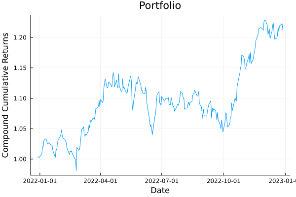
We can also plot the risk contribution per asset. For this, we must provide an instance of the risk measure we want to use with the appropriate statistics/parameters. We can do this by using the factory function (recommended when doing so programmatically), or manually set the quantities ourselves.
# Plot the risk contribution per asset.plot_risk_contribution(factory(Variance(), res.pr), mip_res.w, rd.X; nx = rd.nx)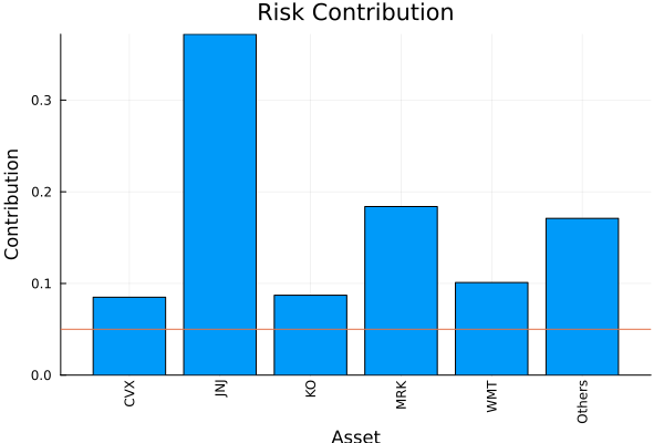
This awkwardness is due to the fact that PortfolioOptimisers.jl tries to decouple the risk measures from optimisation estimators and results. However, the advantage of this approach is that it lets us use multiple different risk measures as part of the risk expression, or as risk limits in optimisations. We explore this further in the examples.
We can plot the histogram of portfolio returns.
# Plot histogram of returns.plot_histogram(mip_res.w, rd.X; slv = slv)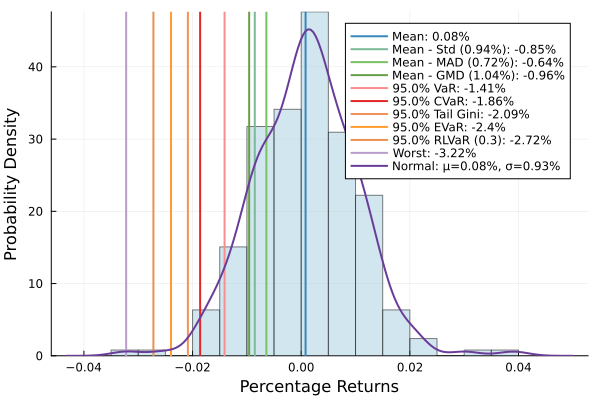
We can also plot the compounded or uncompounded drawdowns.
plot_drawdowns(mip_res.w, rd.X; slv = slv, ts = rd.ts, compound = true)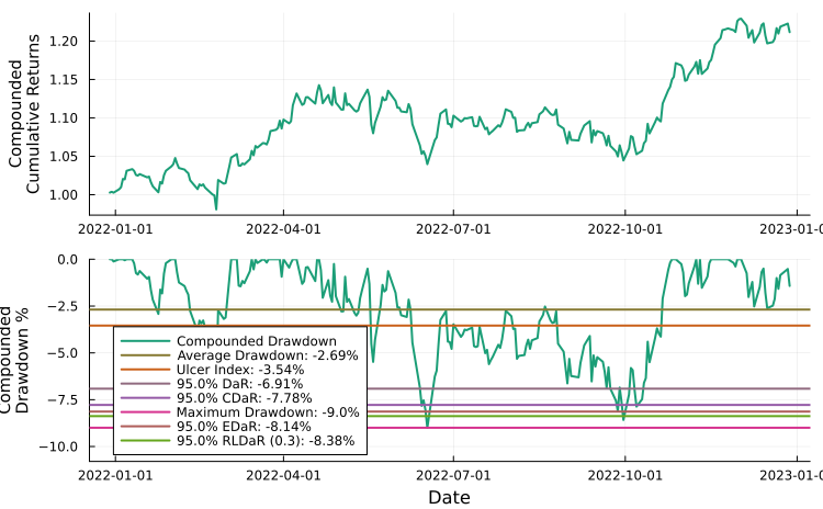
There are many other types of plotting functionality in PortfolioOptimisers.jl, check out the Plotting page of the documentation.