
The source files can be found in examples/.
Finite allocation
An optimiser returns continuous weights — fractions of capital. To actually trade them you need whole shares at real prices under a finite cash budget, and the rounding is not free: it pulls the realised portfolio away from the target, and the smaller the account the more it hurts. PortfolioOptimisers.jl provides two finite-allocation optimisers — a fast solver-free heuristic and an exact mixed-integer one — both called through the same optimise(allocator, FiniteAllocationInput(; w, prices, cash)) interface.
GreedyAllocation— a two-pass heuristic: round to whole (or lot-sized) shares, then spend the leftover cash on the largest underweights. No solver needed.DiscreteAllocation— solves a mixed-integer program for the optimal whole-share book. Needs a MIP solver.
When to reach for this
Reach for finite allocation as the last step before trading, always — continuous weights are not executable. Use GreedyAllocation when you want an instant, dependable answer (and for very large books where the MIP is slow); use DiscreteAllocation when the account is small enough that the rounding genuinely matters and you want the provably best integer book. Watch the realised-vs-target drift — it is your discretisation error.
using PortfolioOptimisers, CSV, TimeSeries, DataFrames, PrettyTables, Clarabel, HiGHS,
      StatsPlots, GraphRecipes

resfmt = (v, i, j) -> begin
    return if j == 1
        v
    else
        isa(v, AbstractFloat) ? "$(round(v*100, digits=3)) %" : v
    end
end;
1. A target portfolio and prices
We optimise a minimum-risk book, then read the latest prices off the price series — finite allocation needs both the target weights and a price per share.
X = TimeArray(CSV.File(joinpath(@__DIR__, "..", "SP500.csv.gz")); timestamp = :Date)[(end - 252):end]
rd = prices_to_returns(X)
pr = prior(EmpiricalPrior(), rd)

slv = Solver(; name = :clarabel, solver = Clarabel.Optimizer,
             settings = Dict("verbose" => false),
             check_sol = (; allow_local = true, allow_almost = true))

res = optimise(MeanRisk(; obj = MinimumRisk(), opt = JuMPOptimiser(; pe = pr, slv = slv)))
prices = vec(values(X)[end, :])
20-element Vector{Float64}:
125.674
62.57
32.301
78.279
173.728
63.883
311.22
174.085
129.575
62.609
363.098
109.581
233.434
179.278
49.25
149.133
24.497
524.422
140.181
106.6272. Greedy allocation
GreedyAllocation needs no solver. The result carries the integer shares, the per-asset cost, the realised weights w, and the leftover cash. With a $100,000 budget the realised weights track the target tightly and only a few dollars go uninvested.
cash = 100_000.0
greedy = optimise(GreedyAllocation(),
                  FiniteAllocationInput(; w = res.w, prices = prices, cash = cash))

drift(alloc) = sum(abs, alloc.w .- res.w)
pretty_table(DataFrame("Asset" => rd.nx, "Target" => res.w,
                       "Shares" => round.(Int, greedy.shares), "Realised" => greedy.w);
             formatters = [resfmt],
             title = "Greedy allocation of \```math(round(Int, cash)) — leftover cash \```(round(greedy.cash, digits = 2)), drift $(round(drift(greedy), digits = 4))")
Greedy allocation of ```math(round(Int, cash)) — leftover cash ```(round(greed ⋯
┌────────┬──────────┬────────┬──────────┐
│ Asset │ Target │ Shares │ Realised │
│ String │ Float64 │ Int64 │ Float64 │
├────────┼──────────┼────────┼──────────┤
│ AAPL │ 0.0 % │ 0 │ 0.0 % │
│ AMD │ 0.0 % │ 0 │ 0.0 % │
│ BAC │ 0.0 % │ 0 │ 0.0 % │
│ BBY │ 0.0 % │ 0 │ 0.0 % │
│ CVX │ 7.432 % │ 43 │ 7.471 % │
│ GE │ 0.806 % │ 13 │ 0.831 % │
│ HD │ 0.0 % │ 0 │ 0.0 % │
│ JNJ │ 36.974 % │ 212 │ 36.911 % │
│ JPM │ 0.749 % │ 6 │ 0.778 % │
│ KO │ 11.161 % │ 178 │ 11.146 % │
│ LLY │ 0.0 % │ 0 │ 0.0 % │
│ MRK │ 17.467 % │ 159 │ 17.426 % │
│ MSFT │ 0.0 % │ 0 │ 0.0 % │
│ PEP │ 8.978 % │ 50 │ 8.965 % │
│ ⋮ │ ⋮ │ ⋮ │ ⋮ │
└────────┴──────────┴────────┴──────────┘
6 rows omitted3. Exact allocation with a MIP solver
DiscreteAllocation solves for the optimal whole-share book instead of a greedy one. It needs a mixed-integer solver — here HiGHS. On a book this size the greedy heuristic is already at (or very near) the optimum, so the two agree; the value of the MIP shows up on tighter budgets and lot constraints where the greedy pass can leave gains on the table.
mip_slv = Solver(; name = :highs, solver = HiGHS.Optimizer,
                 settings = Dict("log_to_console" => false))
discrete = optimise(DiscreteAllocation(; slv = mip_slv),
                    FiniteAllocationInput(; w = res.w, prices = prices, cash = cash))

pretty_table(DataFrame("Method" => ["Greedy", "Discrete (MIP)"],
                       "Leftover cash" => [greedy.cash, discrete.cash],
                       "Drift from target" => [drift(greedy), drift(discrete)]);
             formatters = [resfmt], title = "Greedy vs exact allocation")
Greedy vs exact allocation
┌────────────────┬───────────────┬───────────────────┐
│ Method │ Leftover cash │ Drift from target │
│ String │ Float64 │ Float64 │
├────────────────┼───────────────┼───────────────────┤
│ Greedy │ 1422.3 % │ 0.33 % │
│ Discrete (MIP) │ 1422.3 % │ 0.33 % │
└────────────────┴───────────────┴───────────────────┘4. Lot sizes
Many instruments trade in lots, not single shares. GreedyAllocation(; unit = u) rounds to multiples of u shares. Coarser lots mean a coarser allocation — the drift grows, and a large lot can even overshoot the budget (the leftover cash goes negative), which is the signal that the lot size is too big for the account.
greedy_lots = optimise(GreedyAllocation(; unit = 10),
                       FiniteAllocationInput(; w = res.w, prices = prices, cash = cash))

pretty_table(DataFrame("Allocation" => ["Single shares", "Lots of 10"],
                       "Leftover cash" => [greedy.cash, greedy_lots.cash],
                       "Drift from target" => [drift(greedy), drift(greedy_lots)]);
             formatters = [resfmt], title = "Lot size coarsens the allocation")
Lot size coarsens the allocation
┌───────────────┬───────────────┬───────────────────┐
│ Allocation │ Leftover cash │ Drift from target │
│ String │ Float64 │ Float64 │
├───────────────┼───────────────┼───────────────────┤
│ Single shares │ 1422.3 % │ 0.33 % │
│ Lots of 10 │ -26844.0 % │ 3.388 % │
└───────────────┴───────────────┴───────────────────┘5. Budget size is the discretisation error
The same rounding that is negligible on a large account dominates a small one. Allocating the identical target into $100,000 versus $5,000 shows the drift growing by an order of magnitude — on a small account, the choice of finite-allocation method (and lot size) matters most.
budgets = [100_000.0, 25_000.0, 5_000.0]
budget_allocs = [optimise(GreedyAllocation(),
                          FiniteAllocationInput(; w = res.w, prices = prices, cash = c))
                 for c in budgets]

pretty_table(DataFrame("Budget" => budgets,
                       "Leftover cash" => [a.cash for a in budget_allocs],
                       "Drift from target" => [drift(a) for a in budget_allocs]);
             formatters = [resfmt],
             title = "Smaller budgets suffer larger discretisation error")
Smaller budgets suffer larger discretisation error
┌──────────┬───────────────┬───────────────────┐
│ Budget │ Leftover cash │ Drift from target │
│ Float64 │ Float64 │ Float64 │
├──────────┼───────────────┼───────────────────┤
│ 100000.0 │ 1422.3 % │ 0.33 % │
│ 25000.0 │ 519.1 % │ 1.744 % │
│ 5000.0 │ 536.7 % │ 9.469 % │
└──────────┴───────────────┴───────────────────┘Both allocators also accept a Fees argument, so the share counts can be chosen net of transaction costs (see Fees and Net Returns).
6. Target vs realised
plot_stacked_bar_composition([res, greedy, discrete], rd;
                             xticks = (1:3, ["Target", "Greedy", "Discrete"]))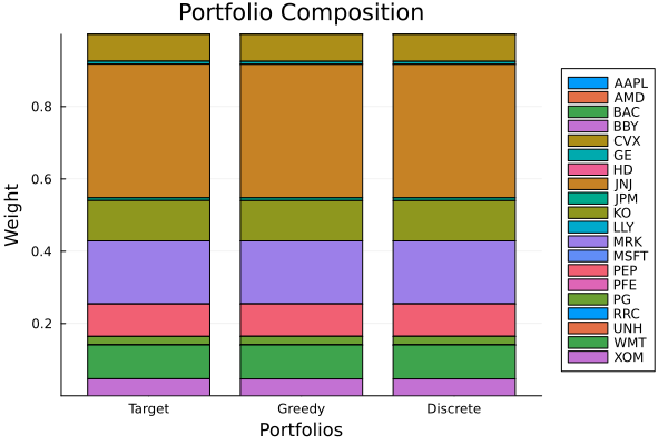
This page was generated using Literate.jl.