The source files can be found in user_guide/.

Post-processing

An optimiser returns continuous weights — fractions of capital. To trade them you need whole shares, and to communicate them you need a report. Post-processing covers both: turning weights into an integer share count under a cash budget, and visualising the result. For the full treatment see the post-processing examples.

using PortfolioOptimisers, CSV, TimeSeries, DataFrames, PrettyTables, Clarabel, StatsPlots,
      GraphRecipes

resfmt = (v, i, j) -> begin
    return if j == 1
        v
    else
        isa(v, AbstractFloat) ? "$(round(v*100, digits=3)) %" : v
    end
end;

X = TimeArray(CSV.File(joinpath(@__DIR__, "../examples/SP500.csv.gz")); timestamp = :Date)[(end - 252):end]
rd = prices_to_returns(X)
pr = prior(EmpiricalPrior(), rd)

slv = Solver(; name = :clarabel, solver = Clarabel.Optimizer,
             settings = Dict("verbose" => false),
             check_sol = (; allow_local = true, allow_almost = true))

res = optimise(MeanRisk(; obj = MinimumRisk(), opt = JuMPOptimiser(; pe = pr, slv = slv)))

MeanRiskResult
  jr ┼ JuMPOptimisationResult
     │        pa ┼ ProcessedJuMPOptimiserAttributes
     │           │        pr ┼ LowOrderPrior
     │           │           │         X ┼ 252×20 Matrix{Float64}
     │           │           │        mu ┼ 20-element Vector{Float64}
     │           │           │     sigma ┼ 20×20 Matrix{Float64}
     │           │           │      chol ┼ nothing
     │           │           │         w ┼ nothing
     │           │           │       ens ┼ nothing
     │           │           │       kld ┼ nothing
     │           │           │        ow ┼ nothing
     │           │           │        rr ┼ nothing
     │           │           │      f_mu ┼ nothing
     │           │           │   f_sigma ┼ nothing
     │           │           │       f_w ┴ nothing
     │           │        wb ┼ WeightBounds
     │           │           │   lb ┼ 20-element StepRangeLen{Float64, Base.TwicePrecision{Float64}, Base.TwicePrecision{Float64}, Int64}
     │           │           │   ub ┴ 20-element StepRangeLen{Float64, Base.TwicePrecision{Float64}, Base.TwicePrecision{Float64}, Int64}
     │           │        lt ┼ nothing
     │           │        st ┼ nothing
     │           │      lcsr ┼ nothing
     │           │       ctr ┼ nothing
     │           │    gcardr ┼ nothing
     │           │   sgcardr ┼ nothing
     │           │      smtx ┼ nothing
     │           │     sgmtx ┼ nothing
     │           │       slt ┼ nothing
     │           │       sst ┼ nothing
     │           │      sglt ┼ nothing
     │           │      sgst ┼ nothing
     │           │        tn ┼ nothing
     │           │      fees ┼ nothing
     │           │       plr ┼ nothing
     │           │       ret ┼ ArithmeticReturn
     │           │           │   ucs ┼ nothing
     │           │           │    lb ┼ nothing
     │           │           │    mu ┴ 20-element Vector{Float64}
     │   retcode ┼ OptimisationSuccess
     │           │   res ┴ Dict{Any, Any}: Dict{Any, Any}()
     │       sol ┼ JuMPOptimisationSolution
     │           │   w ┴ 20-element Vector{Float64}
     │     model ┼ A JuMP Model
     │           │ ├ solver: Clarabel
     │           │ ├ objective_sense: MIN_SENSE
     │           │ │ └ objective_function_type: QuadExpr
     │           │ ├ num_variables: 21
     │           │ ├ num_constraints: 4
     │           │ │ ├ AffExpr in MOI.EqualTo{Float64}: 1
     │           │ │ ├ Vector{AffExpr} in MOI.Nonnegatives: 1
     │           │ │ ├ Vector{AffExpr} in MOI.Nonpositives: 1
     │           │ │ └ Vector{AffExpr} in MOI.SecondOrderCone: 1
     │           │ └ Names registered in the model
     │           │   └ :G, :bgt, :dev_1, :dev_1_soc, :k, :lw, :obj_expr, :ret, :risk, :risk_vec, :sc, :so, :variance_flag, :variance_risk_1, :w, :w_lb, :w_ub
  fb ┴ nothing

1. Finite allocation

Finite allocation converts the continuous weights into integer share counts you can actually buy, given the latest prices and a cash budget. GreedyAllocation is the solver-free option: it rounds to whole shares and spends the leftover cash on the largest underweights. The call takes the weights, the price vector, and the available cash.

prices = vec(values(X)[end, :])
cash = 100_000.0
alloc = optimise(GreedyAllocation(),
                 FiniteAllocationInput(; w = res.w, prices = prices, cash = cash))

GreedyAllocationResult
  retcode ┼ OptimisationSuccess
          │   res ┴ nothing
   shares ┼ 20-element SubArray{Float64, 1, Matrix{Float64}, Tuple{Base.Slice{Base.OneTo{Int64}}, Int64}, true}
     cost ┼ 20-element SubArray{Float64, 1, Matrix{Float64}, Tuple{Base.Slice{Base.OneTo{Int64}}, Int64}, true}
        w ┼ 20-element SubArray{Float64, 1, Matrix{Float64}, Tuple{Base.Slice{Base.OneTo{Int64}}, Int64}, true}
     cash ┼ Float64: 14.223000000023553
       fb ┴ nothing

The result carries the integer shares, the per-asset cost, the realised weights w (after rounding), and the leftover cash. The realised weights track the target closely, and only a few dollars are left uninvested.

invested = sum(alloc.shares .* prices)
pretty_table(DataFrame("Asset" => rd.nx, "Target weight" => res.w,
                       "Shares" => round.(Int, alloc.shares), "Realised weight" => alloc.w);
             formatters = [resfmt],
             title = "Discrete allocation of \```math(round(Int, cash)) — invested \```(round(Int, invested)), cash left \$$(round(alloc.cash, digits = 2))")

Discrete allocation of ```math(round(Int, cash)) — invested ```(round(Int, inv ⋯
┌────────┬───────────────┬────────┬─────────────────┐
│  Asset │ Target weight │ Shares │ Realised weight │
│ String │       Float64 │  Int64 │         Float64 │
├────────┼───────────────┼────────┼─────────────────┤
│   AAPL │         0.0 % │      0 │           0.0 % │
│    AMD │         0.0 % │      0 │           0.0 % │
│    BAC │         0.0 % │      0 │           0.0 % │
│    BBY │         0.0 % │      0 │           0.0 % │
│    CVX │       7.432 % │     43 │         7.471 % │
│     GE │       0.806 % │     13 │         0.831 % │
│     HD │         0.0 % │      0 │           0.0 % │
│    JNJ │      36.974 % │    212 │        36.911 % │
│    JPM │       0.749 % │      6 │         0.778 % │
│     KO │      11.161 % │    178 │        11.146 % │
│    LLY │         0.0 % │      0 │           0.0 % │
│    MRK │      17.467 % │    159 │        17.426 % │
│   MSFT │         0.0 % │      0 │           0.0 % │
│    PEP │       8.978 % │     50 │         8.965 % │
│      ⋮ │             ⋮ │      ⋮ │               ⋮ │
└────────┴───────────────┴────────┴─────────────────┘
                                       6 rows omitted

For an exact (rather than greedy) allocation, DiscreteAllocation solves a mixed-integer program — pass it a MIP-capable Solver. It is more precise but needs a MIP solver; the greedy method needs none. See Finite Allocation.

2. Reporting

The plotting functions used throughout this guide are the reporting toolkit: plot_stacked_bar_composition for weights, plot_measures for risk/return scatters and frontiers, plot_risk_contribution for where the risk sits, and plot_prior for the input moments. Here is the realised portfolio's composition.

plot_stacked_bar_composition([res], rd; xticks = (1:1, ["Min risk"]))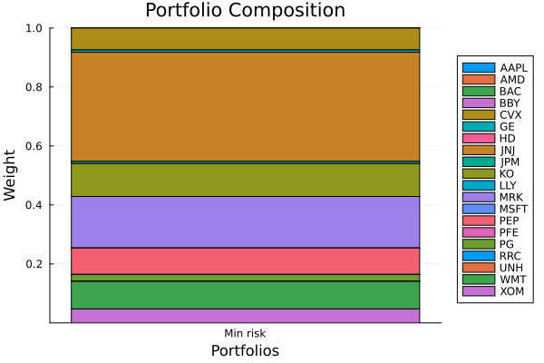

---

This page was generated using Literate.jl.