
The source files can be found in examples/.
Phylogeny and centrality constraints
The constraints in Linear and group constraints act on names and hand-drawn groups. Phylogeny and centrality constraints act on the structure of the asset network instead — the graph of how assets co-move. Rather than telling the optimiser "tech ≤ 30%", you tell it "don't pile into a tightly-knit cluster" or "tilt toward (away from) the hubs of the correlation network". The groups are discovered from the data, not declared.
PortfolioOptimisers.jl builds the network with a NetworkEstimator (or a clustering estimator) and then exposes two families:
Phylogeny constraints (
SemiDefinitePhylogenyEstimator,IntegerPhylogenyEstimator) via theplekeyword — limit joint exposure to network-linked assets.Centrality constraints (
CentralityConstraintbuilt from aCentralityEstimator) via thectekeyword — bound the portfolio's average network centrality.
When to reach for this
Reach for these when your diversification concern is structural rather than by label: you do not want a book that looks diversified by sector but is actually one big correlated bet, or you want to deliberately tilt toward stable hubs or peripheral diversifiers. They need no hand-built groups — the structure comes from the covariance. The semidefinite phylogeny and centrality forms are convex; the integer phylogeny form needs a MIP solver.
using PortfolioOptimisers, CSV, TimeSeries, DataFrames, PrettyTables, Clarabel, StatsPlots,
      GraphRecipes

resfmt = (v, i, j) -> begin
    return if j == 1
        v
    else
        isa(v, AbstractFloat) ? "$(round(v*100, digits=3)) %" : v
    end
end;
1. ReturnsResult data
X = TimeArray(CSV.File(joinpath(@__DIR__, "..", "SP500.csv.gz")); timestamp = :Date)[(end - 252):end]
rd = prices_to_returns(X)
pr = prior(EmpiricalPrior(), rd)

slv = Solver(; name = :clarabel, solver = Clarabel.Optimizer,
             settings = Dict("verbose" => false),
             check_sol = (; allow_local = true, allow_almost = true))

res_base = optimise(MeanRisk(; obj = MinimumRisk(),
                             opt = JuMPOptimiser(; pe = pr, slv = slv)))
MeanRiskResult
jr ┼ JuMPOptimisationResult
│ pa ┼ ProcessedJuMPOptimiserAttributes
│ │ pr ┼ LowOrderPrior
│ │ │ X ┼ 252×20 Matrix{Float64}
│ │ │ mu ┼ 20-element Vector{Float64}
│ │ │ sigma ┼ 20×20 Matrix{Float64}
│ │ │ chol ┼ nothing
│ │ │ w ┼ nothing
│ │ │ ens ┼ nothing
│ │ │ kld ┼ nothing
│ │ │ ow ┼ nothing
│ │ │ rr ┼ nothing
│ │ │ f_mu ┼ nothing
│ │ │ f_sigma ┼ nothing
│ │ │ f_w ┴ nothing
│ │ wb ┼ WeightBounds
│ │ │ lb ┼ 20-element StepRangeLen{Float64, Base.TwicePrecision{Float64}, Base.TwicePrecision{Float64}, Int64}
│ │ │ ub ┴ 20-element StepRangeLen{Float64, Base.TwicePrecision{Float64}, Base.TwicePrecision{Float64}, Int64}
│ │ lt ┼ nothing
│ │ st ┼ nothing
│ │ lcsr ┼ nothing
│ │ ctr ┼ nothing
│ │ gcardr ┼ nothing
│ │ sgcardr ┼ nothing
│ │ smtx ┼ nothing
│ │ sgmtx ┼ nothing
│ │ slt ┼ nothing
│ │ sst ┼ nothing
│ │ sglt ┼ nothing
│ │ sgst ┼ nothing
│ │ tn ┼ nothing
│ │ fees ┼ nothing
│ │ plr ┼ nothing
│ │ ret ┼ ArithmeticReturn
│ │ │ ucs ┼ nothing
│ │ │ lb ┼ nothing
│ │ │ mu ┴ 20-element Vector{Float64}
│ retcode ┼ OptimisationSuccess
│ │ res ┴ Dict{Any, Any}: Dict{Any, Any}()
│ sol ┼ JuMPOptimisationSolution
│ │ w ┴ 20-element Vector{Float64}
│ model ┼ A JuMP Model
│ │ ├ solver: Clarabel
│ │ ├ objective_sense: MIN_SENSE
│ │ │ └ objective_function_type: QuadExpr
│ │ ├ num_variables: 21
│ │ ├ num_constraints: 4
│ │ │ ├ AffExpr in MOI.EqualTo{Float64}: 1
│ │ │ ├ Vector{AffExpr} in MOI.Nonnegatives: 1
│ │ │ ├ Vector{AffExpr} in MOI.Nonpositives: 1
│ │ │ └ Vector{AffExpr} in MOI.SecondOrderCone: 1
│ │ └ Names registered in the model
│ │ └ :G, :bgt, :dev_1, :dev_1_soc, :k, :lw, :obj_expr, :ret, :risk, :risk_vec, :sc, :so, :variance_flag, :variance_risk_1, :w, :w_lb, :w_ub
fb ┴ nothing2. The asset network
A NetworkEstimator turns the covariance into a graph: assets are nodes, and edges link assets whose returns are connected after filtering out the noisy links (a minimum-spanning-tree or similar backbone). Both constraint families below read this graph. You do not have to build it by hand — the estimators take a NetworkEstimator() and construct it from the prior internally.
3. Phylogeny constraints
A SemiDefinitePhylogenyEstimator adds a semidefinite constraint that discourages holding assets which are neighbours in the network — concentrated, mutually-correlated bets. Passing it through ple reshapes the minimum-risk portfolio toward combinations that are diversified in network terms, not just in count.
res_phylo = optimise(MeanRisk(; obj = MinimumRisk(),
                              opt = JuMPOptimiser(; pe = pr, slv = slv,
                                                  ple = SemiDefinitePhylogenyEstimator(;
                                                                                       pl = NetworkEstimator()))))

pretty_table(DataFrame("Asset" => rd.nx, "Baseline" => res_base.w,
                       "Phylogeny" => res_phylo.w); formatters = [resfmt],
             title = "Minimum risk: baseline vs network-phylogeny constrained")
Minimum risk: baseline vs network-phylogeny constrained
┌────────┬──────────┬───────────┐
│ Asset │ Baseline │ Phylogeny │
│ String │ Float64 │ Float64 │
├────────┼──────────┼───────────┤
│ AAPL │ 0.0 % │ 0.0 % │
│ AMD │ 0.0 % │ 0.0 % │
│ BAC │ 0.0 % │ 0.005 % │
│ BBY │ 0.0 % │ 0.0 % │
│ CVX │ 7.432 % │ 12.063 % │
│ GE │ 0.806 % │ 0.109 % │
│ HD │ 0.0 % │ 0.001 % │
│ JNJ │ 36.974 % │ 52.972 % │
│ JPM │ 0.749 % │ 1.95 % │
│ KO │ 11.161 % │ 21.12 % │
│ LLY │ 0.0 % │ 0.001 % │
│ MRK │ 17.467 % │ 0.024 % │
│ MSFT │ 0.0 % │ 0.001 % │
│ PEP │ 8.978 % │ 0.029 % │
│ ⋮ │ ⋮ │ ⋮ │
└────────┴──────────┴───────────┘
6 rows omittedThe constraint moves a large fraction of the book — it is enforcing genuine structural diversification, not a cosmetic tweak. For a hard limit on the number of names drawn from each network cluster, IntegerPhylogenyEstimator imposes an integer (cardinality-style) version; being combinatorial it needs a MIP solver (see Budget Constraints for the Pajarito/HiGHS setup).
4. Centrality constraints
Centrality measures how central each asset is in the network — a hub that co-moves with many others, versus a periphery name that diversifies. A CentralityEstimator scores every asset, and a CentralityConstraint bounds the portfolio's weighted-average centrality through cte. You can push the book toward hubs (comp = >=, a higher floor) or toward the periphery (comp = <=, a lower ceiling).
res_hub = optimise(MeanRisk(; obj = MinimumRisk(),
                            opt = JuMPOptimiser(; pe = pr, slv = slv,
                                                cte = CentralityConstraint(;
                                                                           A = CentralityEstimator(),
                                                                           B = 0.20,
                                                                           comp = >=))))
res_periph = optimise(MeanRisk(; obj = MinimumRisk(),
                               opt = JuMPOptimiser(; pe = pr, slv = slv,
                                                   cte = CentralityConstraint(;
                                                                              A = CentralityEstimator(),
                                                                              B = 0.08,
                                                                              comp = <=))))

centrality = centrality_vector(CentralityEstimator(), pr).X
avg_centrality(w) = sum(w .* centrality)
pretty_table(DataFrame("Portfolio" =>
                           ["Baseline", "Hub-tilted (≥ 0.20)", "Periphery (≤ 0.08)"],
                       "Avg centrality" =>
                           [avg_centrality(res_base.w), avg_centrality(res_hub.w),
                            avg_centrality(res_periph.w)]);
             title = "Average network centrality of the portfolio")
Average network centrality of the portfolio
┌─────────────────────┬────────────────┐
│ Portfolio │ Avg centrality │
│ String │ Float64 │
├─────────────────────┼────────────────┤
│ Baseline │ 0.143427 │
│ Hub-tilted (≥ 0.20) │ 0.2 │
│ Periphery (≤ 0.08) │ 0.0799999 │
└─────────────────────┴────────────────┘The constraint binds in both directions — the hub tilt lifts the average centrality to its floor, the periphery tilt drops it to its ceiling. Centrality is not one number: a CentralityEstimator accepts different algorithms (degree, eigenvector, closeness, betweenness, …), each emphasising a different notion of "central", so the right one depends on what kind of connectedness you care about.
5. Comparing the structural constraints
results = [res_base, res_phylo, res_hub, res_periph]
labels = ["Baseline", "Phylogeny", "Hub", "Periphery"]

plot_stacked_bar_composition(results, rd; xticks = (1:length(labels), labels))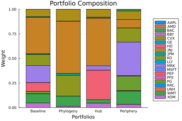
This page was generated using Literate.jl.