PortfolioOptimisers.jlQuantitative portfolio construction
Democratising, demystifying, and derisking investing
Democratising, demystifying, and derisking investing
DANGER
Investing conveys real risk, the entire point of portfolio optimisation is to minimise it to tolerable levels. The examples use outdated data and a variety of stocks (including what I consider to be meme stocks) for demonstration purposes only. None of the information in this documentation should be taken as financial advice. Any advice is limited to improving portfolio construction, most of which is common investment and statistical knowledge.
Portfolio optimisation is the science of either:
Minimising risk whilst keeping returns to acceptable levels.
Maximising returns whilst keeping risk to acceptable levels.
To some definition of acceptable, and with any number of additional constraints available to the optimisation type.
There exist myriad statistical, pre- and post-processing, optimisations, and constraints that allow one to explore an extensive landscape of "optimal" portfolios.
PortfolioOptimisers.jl is an attempt at providing as many of these as possible under a single banner. We make extensive use of Julia's type system, module extensions, and multiple dispatch to simplify development and maintenance.
Please visit the examples and API for details.
PortfolioOptimisers.jl is under active development and still in v0.*.*. Therefore, breaking changes should be expected with v0.X.0 releases. All other releases will fall under v0.X.Y.
The documentation is still under construction.
Testing coverage is still under 95 %. We're mainly missing assertion tests, but some lesser used features are partially or wholly untested.
Please feel free to submit issues, discussions and/or PRs regarding missing docs, examples, features, tests, and bugs.
PortfolioOptimisers.jl is a registered package, so installation is as simple as:
julia> using Pkg

julia> Pkg.add(PackageSpec(; name = "PortfolioOptimisers"))For a roadmap of planned and desired features in no particular order please refer to Issue #37.
Some docstrings are incomplete and/or outdated, please refer to Issue #58 for details on what docstrings have been completed in the dev branch.
The library is quite powerful and extremely flexible. Here is what a very basic end-to-end workflow can look like. The examples contain more thorough explanations and demos. The API docs contain toy examples of the many, many features.
First we import the packages we will need for the example.
StatsPlots and GraphRecipes are needed to load the plotting extension.
Clarabel and HiGHS are the optimisers we will use.
YFinance and TimeSeries for downloading and preprocessing price data.
PrettyTables and DataFrames for displaying the results.
# Import module and plotting extension.
using PortfolioOptimisers, StatsPlots, GraphRecipes
# Import optimisers.
using Clarabel, HiGHS
# Download data.
using YFinance, TimeSeries
# Pretty printing.
using PrettyTables, DataFrames

# Format for pretty tables.
fmt1 = (v, i, j) -> begin
    if j == 1
        return Date(v)
    else
        return v
    end
end;
fmt2 = (v, i, j) -> begin
    if j ∈ (1, 2, 3)
        return v
    else
        return isa(v, Number) ? "$(round(v*100, digits=3)) %" : v
    end
end;
For illustration purposes, we will use a set of popular meme stocks. We need to download and set the price data in a format PortfolioOptimisers.jl can consume.
# Function to convert prices to time array.
function stock_price_to_time_array(x)
    # Only get the keys that are not ticker or datetime.
    coln = collect(keys(x))[3:end]
    # Convert the dictionary into a matrix.
    m = hcat([x[k] for k in coln]...)
    return TimeArray(x["timestamp"], m, Symbol.(coln), x["ticker"])
end

# Tickers to download. These are popular meme stocks, use something better.
assets = sort!(["SOUN", "RIVN", "GME", "AMC", "SOFI", "ENVX", "ANVS", "LUNR", "EOSE", "SMR",
                "NVAX", "UPST", "ACHR", "RKLB", "MARA", "LGVN", "LCID", "CHPT", "MAXN",
                "BB"])

# Prices date range.
Date_0 = "2024-01-01"
Date_1 = "2025-10-05"

# Download the price data using YFinance.
prices = get_prices.(assets; startdt = Date_0, enddt = Date_1)
prices = stock_price_to_time_array.(prices)
prices = hcat(prices...)
cidx = colnames(prices)[occursin.(r"adj", string.(colnames(prices)))]
prices = prices[cidx]
TimeSeries.rename!(prices, Symbol.(assets))
pretty_table(prices[(end - 5):end]; formatters = [fmt1])
┌────────────┬─────────┬─────────┬─────────┬─────────┬─────────┬─────────┬──────
│ timestamp │ ACHR │ AMC │ ANVS │ BB │ CHPT │ ENVX │ ⋯
│ DateTime │ Float64 │ Float64 │ Float64 │ Float64 │ Float64 │ Float64 │ Flo ⋯
├────────────┼─────────┼─────────┼─────────┼─────────┼─────────┼─────────┼──────
│ 2025-09-26 │ 9.28 │ 2.89 │ 1.97 │ 4.96 │ 10.84 │ 10.09 │ 1 ⋯
│ 2025-09-29 │ 9.65 │ 3.0 │ 2.04 │ 5.0 │ 11.05 │ 9.97 │ 1 ⋯
│ 2025-09-30 │ 9.58 │ 2.9 │ 2.07 │ 4.88 │ 10.92 │ 9.97 │ 1 ⋯
│ 2025-10-01 │ 9.81 │ 2.95 │ 2.13 │ 4.79 │ 11.63 │ 11.11 │ 1 ⋯
│ 2025-10-02 │ 10.18 │ 3.15 │ 2.23 │ 4.75 │ 11.32 │ 11.65 │ 1 ⋯
│ 2025-10-03 │ 11.57 │ 3.06 │ 2.22 │ 4.5 │ 11.94 │ 11.92 │ ⋯
└────────────┴─────────┴─────────┴─────────┴─────────┴─────────┴─────────┴──────
14 columns omittedNow we can compute our returns by calling prices_to_returns.
# Compute the returns.
rd = prices_to_returns(prices)
ReturnsResult
nx ┼ 20-element Vector{String}
X ┼ 440×20 Matrix{Float64}
nf ┼ nothing
F ┼ nothing
nb ┼ nothing
B ┼ nothing
ts ┼ 440-element Vector{DateTime}
iv ┼ nothing
ivpa ┴ nothingPortfolioOptimisers.jl uses JuMP for handling the optimisation problems, which means it is solver agnostic and therefore does not ship with any pre-installed solver. Solver lets us define the optimiser factory, its solver-specific settings, and JuMP's solution acceptance criteria.
# Define the continuous solver.
slv = Solver(; name = :clarabel1, solver = Clarabel.Optimizer,
             settings = Dict("verbose" => false, "max_step_fraction" => 0.9),
             check_sol = (; allow_local = true, allow_almost = true))
Solver
name ┼ Symbol: :clarabel1
solver ┼ UnionAll: Clarabel.MOIwrapper.Optimizer
settings ┼ Dict{String, Real}: Dict{String, Real}("verbose" => false, "max_step_fraction" => 0.9)
check_sol ┼ @NamedTuple{allow_local::Bool, allow_almost::Bool}: (allow_local = true, allow_almost = true)
add_bridges ┴ Bool: truePortfolioOptimisers.jl implements a number of optimisation types as estimators. All the ones which use mathematical optimisation require a JuMPOptimiser structure which defines general solver constraints. This structure in turn requires an instance (or vector) of Solver.
opt = JuMPOptimiser(; slv = slv);Here we will use the traditional Mean-Risk MeanRisk optimisation estimator, which defaults to the Markowitz optimisation (minimum risk mean-variance optimisation).
# Vanilla (Markowitz) mean risk optimisation.
mr = MeanRisk(; opt = opt)
MeanRisk
opt ┼ JuMPOptimiser
│ pe ┼ EmpiricalPrior
│ │ ce ┼ PortfolioOptimisersCovariance
│ │ │ ce ┼ Covariance
│ │ │ │ me ┼ SimpleExpectedReturns
│ │ │ │ │ w ┴ nothing
│ │ │ │ ce ┼ GeneralCovariance
│ │ │ │ │ ce ┼ SimpleCovariance: SimpleCovariance(true)
│ │ │ │ │ w ┴ nothing
│ │ │ │ alg ┴ Full()
│ │ │ mp ┼ MatrixProcessing
│ │ │ │ pdm ┼ Posdef
│ │ │ │ │ alg ┼ UnionAll: NearestCorrelationMatrix.Newton
│ │ │ │ │ kwargs ┴ @NamedTuple{}: NamedTuple()
│ │ │ │ dn ┼ nothing
│ │ │ │ dt ┼ nothing
│ │ │ │ alg ┼ nothing
│ │ │ │ order ┴ NTuple{4, Symbol}: (:pdm, :dn, :dt, :alg)
│ │ me ┼ SimpleExpectedReturns
│ │ │ w ┴ nothing
│ │ horizon ┴ nothing
│ slv ┼ Solver
│ │ name ┼ Symbol: :clarabel1
│ │ solver ┼ UnionAll: Clarabel.MOIwrapper.Optimizer
│ │ settings ┼ Dict{String, Real}: Dict{String, Real}("verbose" => false, "max_step_fraction" => 0.9)
│ │ check_sol ┼ @NamedTuple{allow_local::Bool, allow_almost::Bool}: (allow_local = true, allow_almost = true)
│ │ add_bridges ┴ Bool: true
│ wb ┼ WeightBounds
│ │ lb ┼ Float64: 0.0
│ │ ub ┴ Float64: 1.0
│ bgt ┼ Float64: 1.0
│ sbgt ┼ nothing
│ lt ┼ nothing
│ st ┼ nothing
│ lcse ┼ nothing
│ cte ┼ nothing
│ gcarde ┼ nothing
│ sgcarde ┼ nothing
│ smtx ┼ nothing
│ sgmtx ┼ nothing
│ slt ┼ nothing
│ sst ┼ nothing
│ sglt ┼ nothing
│ sgst ┼ nothing
│ tn ┼ nothing
│ fees ┼ nothing
│ sets ┼ nothing
│ tr ┼ nothing
│ ple ┼ nothing
│ ret ┼ ArithmeticReturn
│ │ ucs ┼ nothing
│ │ lb ┼ nothing
│ │ mu ┴ nothing
│ sca ┼ SumScalariser()
│ ccnt ┼ nothing
│ cobj ┼ nothing
│ sc ┼ Int64: 1
│ so ┼ Int64: 1
│ ss ┼ nothing
│ card ┼ nothing
│ scard ┼ nothing
│ nea ┼ nothing
│ l1 ┼ nothing
│ l2 ┼ nothing
│ linf ┼ nothing
│ lp ┼ nothing
│ brt ┼ Bool: false
│ cle_pr ┼ Bool: true
│ strict ┴ Bool: false
r ┼ Variance
│ settings ┼ RiskMeasureSettings
│ │ scale ┼ Float64: 1.0
│ │ ub ┼ nothing
│ │ rke ┴ Bool: true
│ sigma ┼ nothing
│ chol ┼ nothing
│ rc ┼ nothing
│ alg ┴ SquaredSOCRiskExpr()
obj ┼ MinimumRisk()
wi ┼ nothing
fb ┴ nothingAs you can see, there are a lot of fields in this structure, which correspond to a wide variety of optimisation constraints. We will explore these in the examples. For now, we will perform the optimisation via optimise.
# Perform the optimisation, res.w contains the optimal weights.
res = optimise(mr, rd)
MeanRiskResult
jr ┼ JuMPOptimisationResult
│ oe ┼ DataType: DataType
│ pa ┼ ProcessedJuMPOptimiserAttributes
│ │ pr ┼ LowOrderPrior
│ │ │ X ┼ 440×20 Matrix{Float64}
│ │ │ mu ┼ 20-element Vector{Float64}
│ │ │ sigma ┼ 20×20 Matrix{Float64}
│ │ │ chol ┼ nothing
│ │ │ w ┼ nothing
│ │ │ ens ┼ nothing
│ │ │ kld ┼ nothing
│ │ │ ow ┼ nothing
│ │ │ rr ┼ nothing
│ │ │ f_mu ┼ nothing
│ │ │ f_sigma ┼ nothing
│ │ │ f_w ┴ nothing
│ │ wb ┼ WeightBounds
│ │ │ lb ┼ 20-element StepRangeLen{Float64, Base.TwicePrecision{Float64}, Base.TwicePrecision{Float64}, Int64}
│ │ │ ub ┴ 20-element StepRangeLen{Float64, Base.TwicePrecision{Float64}, Base.TwicePrecision{Float64}, Int64}
│ │ lt ┼ nothing
│ │ st ┼ nothing
│ │ lcsr ┼ nothing
│ │ ctr ┼ nothing
│ │ gcardr ┼ nothing
│ │ sgcardr ┼ nothing
│ │ smtx ┼ nothing
│ │ sgmtx ┼ nothing
│ │ slt ┼ nothing
│ │ sst ┼ nothing
│ │ sglt ┼ nothing
│ │ sgst ┼ nothing
│ │ tn ┼ nothing
│ │ fees ┼ nothing
│ │ plr ┼ nothing
│ │ ret ┼ ArithmeticReturn
│ │ │ ucs ┼ nothing
│ │ │ lb ┼ nothing
│ │ │ mu ┴ 20-element Vector{Float64}
│ retcode ┼ OptimisationSuccess
│ │ res ┴ Dict{Any, Any}: Dict{Any, Any}()
│ sol ┼ JuMPOptimisationSolution
│ │ w ┴ 20-element Vector{Float64}
│ model ┼ A JuMP Model
│ │ ├ solver: Clarabel
│ │ ├ objective_sense: MIN_SENSE
│ │ │ └ objective_function_type: QuadExpr
│ │ ├ num_variables: 21
│ │ ├ num_constraints: 4
│ │ │ ├ AffExpr in MOI.EqualTo{Float64}: 1
│ │ │ ├ Vector{AffExpr} in MOI.Nonnegatives: 1
│ │ │ ├ Vector{AffExpr} in MOI.Nonpositives: 1
│ │ │ └ Vector{AffExpr} in MOI.SecondOrderCone: 1
│ │ └ Names registered in the model
│ │ └ :G, :bgt, :dev_1, :dev_1_soc, :k, :lw, :obj_expr, :ret, :risk, :risk_vec, :sc, :so, :variance_flag, :variance_risk_1, :w, :w_lb, :w_ub
fb ┴ nothingThe solution lives in the sol field, but the weights can be accessed via the w property.
PortfolioOptimisers.jl also has the capability to perform finite allocations, which is useful for those of us without infinite money. There are two ways to do so, a greedy algorithm GreedyAllocation that does not guarantee optimality but is fast and always converges, and a discrete allocation DiscreteAllocation which uses mixed-integer programming (MIP) and requires a capable solver.
Here we will use the latter.
# Define the MIP solver for finite discrete allocation.
mip_slv = Solver(; name = :highs1, solver = HiGHS.Optimizer,
                 settings = Dict("log_to_console" => false),
                 check_sol = (; allow_local = true, allow_almost = true))

# Discrete finite allocation.
da = DiscreteAllocation(; slv = mip_slv)
DiscreteAllocation
slv ┼ Solver
│ name ┼ Symbol: :highs1
│ solver ┼ DataType: DataType
│ settings ┼ Dict{String, Bool}: Dict{String, Bool}("log_to_console" => 0)
│ check_sol ┼ @NamedTuple{allow_local::Bool, allow_almost::Bool}: (allow_local = true, allow_almost = true)
│ add_bridges ┴ Bool: true
sc ┼ Int64: 1
so ┼ Int64: 1
wf ┼ AbsoluteErrorWeightFinaliser()
fb ┼ GreedyAllocation
│ unit ┼ Int64: 1
│ args ┼ Tuple{}: ()
│ kwargs ┼ @NamedTuple{}: NamedTuple()
│ fb ┴ nothingThe discrete allocation minimises the absolute or relative L1- or L2-norm (configurable) between the ideal allocation to the one you can afford plus the leftover cash. As such, it needs to know a few extra things, namely the optimal weights res.w, a vector of the latest prices vec(values(prices[end])), and available cash which we define to be 4206.90.
# Perform the finite discrete allocation, uses the final asset
# prices, and an available cash amount. This is for us mortals
# without infinite wealth.
mip_res = optimise(da, res.w, vec(values(prices[end])), 4206.90)
DiscreteAllocationResult
oe ┼ DataType: DataType
retcode ┼ OptimisationSuccess
│ res ┴ nothing
s_retcode ┼ nothing
l_retcode ┼ OptimisationSuccess
│ res ┴ Dict{Any, Any}: Dict{Any, Any}()
shares ┼ 20-element SubArray{Float64, 1, Matrix{Float64}, Tuple{Base.Slice{Base.OneTo{Int64}}, Int64}, true}
cost ┼ 20-element SubArray{Float64, 1, Matrix{Float64}, Tuple{Base.Slice{Base.OneTo{Int64}}, Int64}, true}
w ┼ 20-element SubArray{Float64, 1, Matrix{Float64}, Tuple{Base.Slice{Base.OneTo{Int64}}, Int64}, true}
cash ┼ Float64: 0.2000379800774681
s_model ┼ nothing
l_model ┼ A JuMP Model
│ ├ solver: HiGHS
│ ├ objective_sense: MIN_SENSE
│ │ └ objective_function_type: AffExpr
│ ├ num_variables: 21
│ ├ num_constraints: 42
│ │ ├ AffExpr in MOI.GreaterThan{Float64}: 1
│ │ ├ Vector{AffExpr} in MOI.NormOneCone: 1
│ │ ├ VariableRef in MOI.GreaterThan{Float64}: 20
│ │ └ VariableRef in MOI.Integer: 20
│ └ Names registered in the model
│ └ :cabs_err, :cr, :r, :sc, :so, :u, :x
fb ┴ nothingWe can display the results in a table.
# View the results.
df = DataFrame(:assets => rd.nx, :shares => mip_res.shares, :cost => mip_res.cost,
               :opt_weights => res.w, :mip_weights => mip_res.w)
pretty_table(df; formatters = [fmt2])
┌────────┬─────────┬─────────┬─────────────┬─────────────┐
│ assets │ shares │ cost │ opt_weights │ mip_weights │
│ String │ Float64 │ Float64 │ Float64 │ Float64 │
├────────┼─────────┼─────────┼─────────────┼─────────────┤
│ ACHR │ 0.0 │ 0.0 │ 0.0 % │ 0.0 % │
│ AMC │ 73.0 │ 223.38 │ 5.324 % │ 5.31 % │
│ ANVS │ 22.0 │ 48.84 │ 1.249 % │ 1.161 % │
│ BB │ 273.0 │ 1228.5 │ 29.184 % │ 29.203 % │
│ CHPT │ 11.0 │ 131.34 │ 3.002 % │ 3.122 % │
│ ENVX │ 0.0 │ 0.0 │ 0.0 % │ 0.0 % │
│ EOSE │ 8.0 │ 100.8 │ 2.435 % │ 2.396 % │
│ GME │ 0.0 │ 0.0 │ 0.0 % │ 0.0 % │
│ LCID │ 1.0 │ 24.77 │ 0.638 % │ 0.589 % │
│ LGVN │ 325.0 │ 256.1 │ 6.089 % │ 6.088 % │
│ LUNR │ 0.0 │ 0.0 │ 0.0 % │ 0.0 % │
│ MARA │ 1.0 │ 18.82 │ 0.613 % │ 0.447 % │
│ MAXN │ 0.0 │ 0.0 │ 0.0 % │ 0.0 % │
│ NVAX │ 28.0 │ 264.88 │ 6.21 % │ 6.297 % │
│ RIVN │ 55.0 │ 750.75 │ 17.897 % │ 17.847 % │
│ ⋮ │ ⋮ │ ⋮ │ ⋮ │ ⋮ │
└────────┴─────────┴─────────┴─────────────┴─────────────┘
5 rows omittedWe can also visualise the portfolio using various plotting functions. For example, we can plot the portfolio's cumulative returns, in this case compound returns.
# Plot the portfolio cumulative returns of the finite allocation portfolio.
plot_ptf_cumulative_returns(mip_res.w, rd.X; ts = rd.ts, compound = true)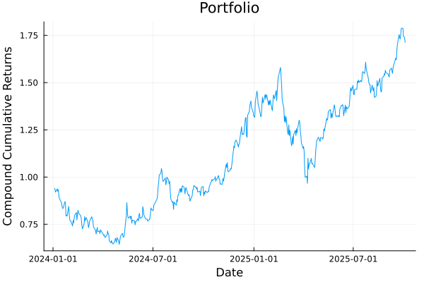
We can also plot the risk contribution per asset. For this, we must provide an instance of the risk measure we want to use with the appropriate statistics/parameters. We can do this by using the factory function (recommended when doing so programmatically), or manually set the quantities ourselves.
# Plot the risk contribution per asset.
plot_risk_contribution(factory(Variance(), res.pr), mip_res.w, rd.X; nx = rd.nx)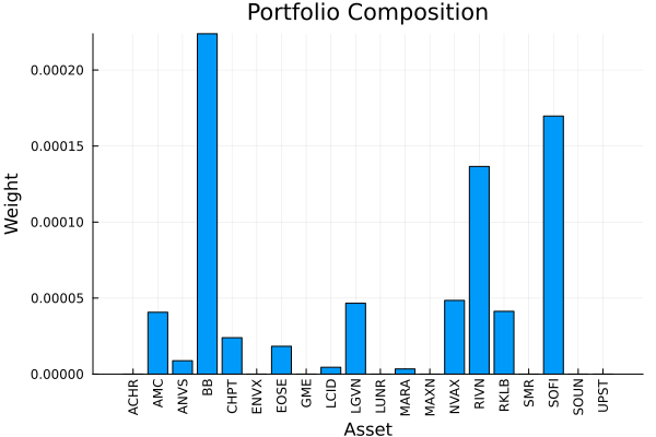
This awkwardness is due to the fact that PortfolioOptimisers.jl tries to decouple the risk measures from optimisation estimators and results. However, the advantage of this approach is that it lets us use multiple different risk measures as part of the risk expression, or as risk limits in optimisations. We explore this further in the examples.
We can plot the histogram of portfolio returns.
# Plot histogram of returns.
plot_histogram(mip_res.w, rd.X; slv = slv)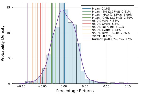
We can also plot the compounded or uncompounded drawdowns.
plot_drawdowns(mip_res.w, rd.X; slv = slv, ts = rd.ts, compound = true)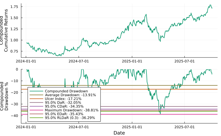
There are many other types of plotting functionality in PortfolioOptimisers.jl, check out the Plotting page of the documentation.
 Daniel Celis Garza