
The source files can be found in examples/.
Cardinality and threshold
This example walks from the simplest mixed-integer constraints to the most structured ones: 2. Asset-level cardinality and buy-in thresholds: card, lt, st.
Group cardinality over assets:
gcarde.Set-level cardinality and thresholds:
scard,slt,sstwithsmtx.Group-of-sets cardinality and thresholds:
sgcarde,sglt,sgstwithsgmtx.
The core idea is simple: constraints become more structured as you move from assets to sets to groups of sets.
When to reach for this
Reach for cardinality and threshold constraints when the number of positions matters as much as their sizes — enforcing a maximum count of holdings, a minimum buy-in so you never take dust positions, or limits on how many names, sets, or groups can be active. These are the tools for turning a dense optimiser solution into an implementable, sparse portfolio.
MIP required
These constraints introduce binary variables, so they need a mixed-integer-capable solver.
using PortfolioOptimisers, CSV, TimeSeries, DataFrames, PrettyTables, Clarabel, HiGHS,
      Pajarito, JuMP, StatsPlots, GraphRecipes

resfmt = (v, i, j) -> begin
    if j == 1
        return v
    else
        return isa(v, Number) ? "$(round(v * 100, digits = 3)) %" : v
    end
end
#2 (generic function with 1 method)1. Setup
We use the same S&P 500 slice as the rest of the examples, but with the exact asset-set fixtures that make the cardinality examples easy to read and, more importantly, feasible.
X = TimeArray(CSV.File(joinpath(@__DIR__, "..", "SP500.csv.gz")); timestamp = :Date)[(end - 252):end]
rd = prices_to_returns(X)
pr = prior(HighOrderPriorEstimator(), rd)
rf = 4.2 / 100 / 252

slv = [Solver(; name = :clarabel1, solver = Clarabel.Optimizer,
              check_sol = (; allow_local = true, allow_almost = true),
              settings = Dict("verbose" => false)),
       Solver(; name = :clarabel2, solver = Clarabel.Optimizer,
              check_sol = (; allow_local = true, allow_almost = true),
              settings = Dict("verbose" => false, "max_step_fraction" => 0.95)),
       Solver(; name = :clarabel3, solver = Clarabel.Optimizer,
              check_sol = (; allow_local = true, allow_almost = true),
              settings = Dict("verbose" => false, "max_step_fraction" => 0.9)),
       Solver(; name = :clarabel4, solver = Clarabel.Optimizer,
              check_sol = (; allow_local = true, allow_almost = true),
              settings = Dict("verbose" => false, "max_step_fraction" => 0.85))]

mip_slv = [Solver(; name = :mip1,
                  solver = optimizer_with_attributes(Pajarito.Optimizer, "verbose" => false,
                                                     "oa_solver" =>
                                                         optimizer_with_attributes(HiGHS.Optimizer,
                                                                                   JuMP.MOI.Silent() =>
                                                                                       true),
                                                     "conic_solver" =>
                                                         optimizer_with_attributes(Clarabel.Optimizer,
                                                                                   "verbose" =>
                                                                                       false)),
                  check_sol = (; allow_local = true, allow_almost = true)),
           Solver(; name = :mip2,
                  solver = optimizer_with_attributes(Pajarito.Optimizer, "verbose" => false,
                                                     "oa_solver" =>
                                                         optimizer_with_attributes(HiGHS.Optimizer,
                                                                                   JuMP.MOI.Silent() =>
                                                                                       true),
                                                     "conic_solver" =>
                                                         optimizer_with_attributes(Clarabel.Optimizer,
                                                                                   "verbose" =>
                                                                                       false,
                                                                                   "max_step_fraction" =>
                                                                                       0.95)),
                  check_sol = (; allow_local = true, allow_almost = true))]

sets = AssetSets(;
                 dict = Dict("nx" => rd.nx, "group1" => rd.nx[1:2:end],
                             "group2" => rd.nx[2:2:end],
                             "clusters1" =>
                                 [1, 1, 1, 1, 1, 1, 1, 2, 2, 2, 2, 2, 2, 2, 3, 3, 3, 3, 3,
                                  3],
                             "clusters2" =>
                                 [1, 2, 3, 1, 2, 3, 1, 2, 3, 1, 2, 3, 1, 2, 3, 1, 2, 3, 1,
                                  2], "c1" => rd.nx[1:3:end], "c2" => rd.nx[2:3:end],
                             "c3" => rd.nx[3:3:end],
                             "nx_industries" => ["Technology", "Technology", "Financials",
                                                 "Consumer_Discretionary", "Energy", "Industrials",
                                                 "Consumer_Discretionary", "Healthcare", "Financials",
                                                 "Consumer_Staples", "Healthcare", "Healthcare",
                                                 "Technology", "Consumer_Staples", "Healthcare",
                                                 "Consumer_Staples", "Energy", "Healthcare",
                                                 "Consumer_Staples", "Energy"],
                             "ux_industries" =>
                                 ["Technology", "Financials", "Consumer_Discretionary",
                                  "Energy", "Industrials", "Healthcare",
                                  "Consumer_Staples"]))
AssetSets
key ┼ String: "nx"
ukey ┼ String: "ux"
dict ┴ Dict{String, Vector}: Dict{String, Vector}("c2" => ["AMD", "CVX", "JNJ", "LLY", "PEP", "RRC", "XOM"], "nx" => ["AAPL", "AMD", "BAC", "BBY", "CVX", "GE", "HD", "JNJ", "JPM", "KO", "LLY", "MRK", "MSFT", "PEP", "PFE", "PG", "RRC", "UNH", "WMT", "XOM"], "c1" => ["AAPL", "BBY", "HD", "KO", "MSFT", "PG", "WMT"], "group2" => ["AMD", "BBY", "GE", "JNJ", "KO", "MRK", "PEP", "PG", "UNH", "XOM"], "clusters2" => [1, 2, 3, 1, 2, 3, 1, 2, 3, 1, 2, 3, 1, 2, 3, 1, 2, 3, 1, 2], "nx_industries" => ["Technology", "Technology", "Financials", "Consumer_Discretionary", "Energy", "Industrials", "Consumer_Discretionary", "Healthcare", "Financials", "Consumer_Staples", "Healthcare", "Healthcare", "Technology", "Consumer_Staples", "Healthcare", "Consumer_Staples", "Energy", "Healthcare", "Consumer_Staples", "Energy"], "c3" => ["BAC", "GE", "JPM", "MRK", "PFE", "UNH"], "clusters1" => [1, 1, 1, 1, 1, 1, 1, 2, 2, 2, 2, 2, 2, 2, 3, 3, 3, 3, 3, 3], "ux_industries" => ["Technology", "Financials", "Consumer_Discretionary", "Energy", "Industrials", "Healthcare", "Consumer_Staples"], "group1" => ["AAPL", "BAC", "CVX", "HD", "JPM", "LLY", "MSFT", "PFE", "RRC", "WMT"])2. Asset-level: card, lt, st
card limits the number of significant assets. lt/st are buy-in thresholds on individual long/short positions.
res_card = optimise(MeanRisk(; opt = JuMPOptimiser(; pe = pr, slv = mip_slv, card = 3)))

res_card_l2 = optimise(MeanRisk(; obj = MaximumRatio(; rf = rf),
                                opt = JuMPOptimiser(; l2 = L2Regularisation(; val = 0.1),
                                                    pe = pr, slv = mip_slv, card = 3)))

res_card_thr = optimise(MeanRisk(; obj = MaximumRatio(; rf = rf),
                                 opt = JuMPOptimiser(; pe = pr, slv = mip_slv,
                                                     wb = WeightBounds(; lb = -1, ub = 1),
                                                     sbgt = 1, bgt = 1, card = 7)))

println("Asset-level cardinality")
println("  active assets (card = 3): ", count(res_card.w .> 1e-10))
println("  active assets (l2 + card = 3): ", count(res_card_l2.w .> 1e-10))
println("  active assets with bounds (card = 7): ", count(abs.(res_card_thr.w) .> 1e-10))
pretty_table(DataFrame(:Asset => rd.nx, :w_card => res_card.w, :w_card_l2 => res_card_l2.w,
                       :w_card_bounded => res_card_thr.w); formatters = [resfmt])
┌ Warning: integral solution repeated
└ @ Pajarito ~/.julia/packages/Pajarito/mhMdw/src/algorithms.jl:103
Asset-level cardinality
active assets (card = 3): 3
active assets (l2 + card = 3): 3
active assets with bounds (card = 7): 5
┌────────┬──────────┬───────────┬────────────────┐
│ Asset │ w_card │ w_card_l2 │ w_card_bounded │
│ String │ Float64 │ Float64 │ Float64 │
├────────┼──────────┼───────────┼────────────────┤
│ AAPL │ 0.0 % │ 0.0 % │ -0.0 % │
│ AMD │ 0.0 % │ 0.0 % │ -26.968 % │
│ BAC │ 0.0 % │ 0.0 % │ -0.0 % │
│ BBY │ 0.0 % │ 0.0 % │ -0.0 % │
│ CVX │ 0.0 % │ 30.163 % │ -0.0 % │
│ GE │ 0.0 % │ 0.0 % │ -0.0 % │
│ HD │ 0.0 % │ 0.0 % │ -0.0 % │
│ JNJ │ 0.0 % │ 0.0 % │ -0.0 % │
│ JPM │ 0.0 % │ 0.0 % │ -0.0 % │
│ KO │ 0.0 % │ 0.0 % │ -0.0 % │
│ LLY │ 0.0 % │ 0.0 % │ 37.732 % │
│ MRK │ 59.481 % │ 0.0 % │ 100.0 % │
│ MSFT │ 0.0 % │ 0.0 % │ -0.0 % │
│ PEP │ 0.0 % │ 0.0 % │ -0.0 % │
│ PFE │ 0.0 % │ 0.0 % │ -68.217 % │
│ ⋮ │ ⋮ │ ⋮ │ ⋮ │
└────────┴──────────┴───────────┴────────────────┘
5 rows omitted3. Group cardinality over assets: gcarde
gcarde uses linear group expressions to constrain how many assets in a named group can be active.
res_gcard = optimise(MeanRisk(;
                              opt = JuMPOptimiser(; pe = pr, slv = mip_slv,
                                                  gcarde = LinearConstraintEstimator(;
                                                                                     val = [:(XOM +
                                                                                              MRK +
                                                                                              WMT <=
                                                                                              2),
                                                                                            :(group2 ==
                                                                                              5)]),
                                                  sets = sets)))

println("Group cardinality over assets")
println("  active names in XOM/MRK/WMT group: ",
        count(res_gcard.w[.!iszero.(vec(res_gcard.gcardr.A_ineq[1, :]))] .> 1e-10))
println("  active names in group2: ",
        count(res_gcard.w[.!iszero.(vec(res_gcard.gcardr.A_eq[1, :]))] .> 1e-10))
Group cardinality over assets
active names in XOM/MRK/WMT group: 2
active names in group2: 54. Set-level: scard, slt, sst with smtx
Here the constraints act on the sum of the weights in each set.
smtxmaps assets to sets.scardlimits the number of active sets.slt/sstthreshold the set-level sums.
res_set_1 = optimise(MeanRisk(; r = ConditionalValueatRisk(), obj = MinimumRisk(),
                              opt = JuMPOptimiser(; pe = pr, slv = mip_slv, scard = 1,
                                                  smtx = AssetSetsMatrixEstimator(;
                                                                                  val = "clusters1"),
                                                  sets = sets)), rd)

res_set_2 = optimise(MeanRisk(; r = ConditionalValueatRisk(), obj = MaximumRatio(; rf = rf),
                              opt = JuMPOptimiser(; pe = pr, slv = mip_slv, scard = 2,
                                                  slt = Threshold(; val = fill(0.73, 3)),
                                                  sst = Threshold(; val = 0.38),
                                                  wb = WeightBounds(; lb = -1, ub = 1),
                                                  sbgt = 1, bgt = nothing,
                                                  smtx = AssetSetsMatrixEstimator(;
                                                                                  val = "clusters1"),
                                                  sets = sets)), rd)

set_exposure = res_set_2.smtx * res_set_2.w
println("Set-level cardinality and thresholds")
println("  active sets (scard = 1): ",
        count(.!iszero.([sum(res_set_1.w[res_set_1.smtx[i, :]]) for i in axes(res_set_1.smtx, 1)])))
println("  active sets (scard = 2): ",
        count(.!iszero.([sum(res_set_2.w[res_set_2.smtx[i, :]]) for i in axes(res_set_2.smtx, 1)])))
println("  min set exposure: ", minimum(set_exposure))
println("  max set exposure: ", maximum(set_exposure))
pretty_table(DataFrame(:Set => ["cluster 1", "cluster 2", "cluster 3"],
                       :set_exposure => set_exposure); formatters = [resfmt])
Set-level cardinality and thresholds
active sets (scard = 1): 1
active sets (scard = 2): 3
min set exposure: -0.3800000000000003
max set exposure: 0.7300000000000001
┌───────────┬──────────────┐
│ Set │ set_exposure │
│ String │ Float64 │
├───────────┼──────────────┤
│ cluster 1 │ -38.0 % │
│ cluster 2 │ 73.0 % │
│ cluster 3 │ -0.0 % │
└───────────┴──────────────┘5. Group-of-sets: sgcarde, sglt, sgst with sgmtx
Now the constraints are defined over groups of sets, not directly over assets.
sgmtxmaps assets to set groups.sgcardeconstrains cardinality over those groups.sglt/sgstthreshold grouped set exposures.
Feasibility still depends on the budget and the bounds, so we use the same values as the tested constraint block.
res_sg_1 = optimise(MeanRisk(;
                             opt = JuMPOptimiser(; slv = mip_slv, sets = sets,
                                                 sglt = Threshold(0.015),
                                                 sgcarde = LinearConstraintEstimator(;
                                                                                     key = "ux_industries",
                                                                                     val = [:(ux_industries ==
                                                                                              4)]),
                                                 sgmtx = AssetSetsMatrixEstimator(;
                                                                                  val = "nx_industries"))),
                    rd)

res_sg_2 = optimise(MeanRisk(;
                             opt = JuMPOptimiser(; slv = mip_slv,
                                                 wb = WeightBounds(; lb = -1, ub = 1),
                                                 sbgt = 1, bgt = nothing,
                                                 sglt = [ThresholdEstimator(;
                                                                            val = fill(0.53,
                                                                                       7),
                                                                            key = "ux_industries")],
                                                 sgst = [ThresholdEstimator(;
                                                                            val = fill(0.32,
                                                                                       7),
                                                                            key = "ux_industries")],
                                                 sgcarde = [LinearConstraintEstimator(;
                                                                                      key = "ux_industries",
                                                                                      val = [:(ux_industries >=
                                                                                               4),
                                                                                             :(ux_industries <=
                                                                                               6)])],
                                                 sgmtx = [AssetSetsMatrixEstimator(;
                                                                                   val = "nx_industries")],
                                                 sets = sets)), rd)

group_exposure_1 = res_sg_1.sgmtx * res_sg_1.w
group_exposure_2 = res_sg_2.sgmtx[1] * res_sg_2.w
println("Group-of-sets constraints")
println("  grouped set count (single constraint run): ",
        count(abs.(group_exposure_1) .> 1e-10))
println("  grouped set count (threshold run): ", count(abs.(group_exposure_2) .> 5e-10))
println("  min grouped long exposure: ", minimum(group_exposure_2[group_exposure_2 .> 0]))
println("  max grouped short exposure: ", maximum(group_exposure_2[group_exposure_2 .< 0]))
pretty_table(DataFrame(:GroupSet => sets.dict["ux_industries"],
                       :group_exposure => group_exposure_2); formatters = [resfmt])
Group-of-sets constraints
grouped set count (single constraint run): 4
grouped set count (threshold run): 4
min grouped long exposure: 6.16749083444737e-14
max grouped short exposure: -0.32000040258050805
┌────────────────────────┬────────────────┐
│ GroupSet │ group_exposure │
│ String │ Float64 │
├────────────────────────┼────────────────┤
│ Technology │ -32.0 % │
│ Financials │ 0.0 % │
│ Consumer_Discretionary │ 53.0 % │
│ Energy │ 0.0 % │
│ Industrials │ 0.0 % │
│ Healthcare │ -32.0 % │
│ Consumer_Staples │ -32.0 % │
└────────────────────────┴────────────────┘6. Side-by-side summary
pretty_table(DataFrame("Case" => ["asset card", "asset card + l2", "gcarde", "set-level",
                                  "group-of-sets"],
                       "Active assets" =>
                           [count(res_card.w .> 1e-10), count(res_card_l2.w .> 1e-10),
                            count(res_gcard.w .> 1e-10), count(res_set_1.w .> 1e-10),
                            count(res_sg_1.w .> 1e-10)]))
┌─────────────────┬───────────────┐
│ Case │ Active assets │
│ String │ Int64 │
├─────────────────┼───────────────┤
│ asset card │ 3 │
│ asset card + l2 │ 3 │
│ gcarde │ 15 │
│ set-level │ 4 │
│ group-of-sets │ 14 │
└─────────────────┴───────────────┘7. Composition across constraint families
A final visual comparison of how each constraint family reshapes the allocation: asset-level cardinality collapses to a few names, while the set- and group-level constraints spread the budget across the structure they are defined on.
plot_stacked_bar_composition([res_card, res_card_l2, res_gcard, res_set_1, res_sg_1], rd;
                             xticks = ([1, 2, 3, 4, 5],
                                       ["asset card", "card+l2", "gcarde", "set-level",
                                        "group-of-sets"]))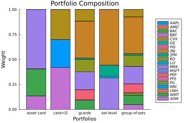
Takeaways:
Use
card,lt,stfor direct asset-level sparsity and buy-in behavior.Use
gcardewhen the constraint is a linear statement over a named asset group.Use
smtx+scard/slt/sstwhen the constraint should apply to set sums.Use
sgmtx+sgcarde/sglt/sgstwhen the constraint should apply to groups of sets.If the solver returns an infeasible or failed retcode, the threshold or cardinality target is too tight for the available budget and bounds.
This page was generated using Literate.jl.