
The source files can be found in examples/.
Opinion pooling
Entropy pooling turns one set of views into a reweighted prior. But in practice you often have several views from different sources — a fundamental analyst, a quant signal, a macro desk — and they may disagree. Opinion pooling combines several entropy-pooling posteriors into a single consensus prior, weighting each opinion by how much you trust it. It is the natural capstone of the view-prior arc: each opinion is itself an EntropyPoolingPrior, and the pool blends them.
PortfolioOptimisers implements it as OpinionPoolingPrior: you pass a vector of entropy-pooling priors as pes, optional credibility weights w, a pooling algorithm (LinearOpinionPooling or LogarithmicOpinionPooling), and an optional robust confidence p. This page is a deep dive: we build three opinions, pool them, then work through every lever the pool exposes — the two pooling algorithms, the credibility weights and their uniform-prior fallback, and robust pooling that automatically discounts outlier opinions.
When to reach for this
Reach for opinion pooling when you have multiple, possibly conflicting, sets of views and want a principled consensus rather than picking a winner or hand-averaging forecasts. Assign each opinion a weight reflecting its credibility; the pool degrades gracefully when opinions disagree. If you only have a single coherent set of views, plain entropy pooling is enough; if your views are mean-only and Gaussian, Black–Litterman is lighter still.
using PortfolioOptimisers, PrettyTables

mmtfmt = (v, i, j) -> begin
    if j == 1
        return v
    else
        return isa(v, Number) ? "$(round(v*100, digits=4)) %" : v
    end
end;
resfmt = (v, i, j) -> begin
    if j == 1
        return v
    else
        return isa(v, Number) ? "$(round(v*100, digits=3)) %" : v
    end
end;
1. ReturnsResult data
We use the same S&P 500 slice as the other examples.
using CSV, TimeSeries, DataFrames

X = TimeArray(CSV.File(joinpath(@__DIR__, "..", "SP500.csv.gz")); timestamp = :Date)[(end - 252):end]
rd = prices_to_returns(X)

sets = AssetSets(;
                 dict = Dict("nx" => rd.nx, "tech" => ["AAPL", "AMD", "MSFT"],
                             "energy" => ["CVX"]))
AssetSets
key ┼ String: "nx"
ukey ┼ String: "ux"
dict ┴ Dict{String, Vector{String}}: Dict("nx" => ["AAPL", "AMD", "BAC", "BBY", "CVX", "GE", "HD", "JNJ", "JPM", "KO", "LLY", "MRK", "MSFT", "PEP", "PFE", "PG", "RRC", "UNH", "WMT", "XOM"], "tech" => ["AAPL", "AMD", "MSFT"], "energy" => ["CVX"])2. Three opinions
Each opinion is an EntropyPoolingPrior with its own views — think of them as three analysts who looked at the same market and came to different conclusions:
Opinion A (bullish Apple):
AAPL == 0.0008.Opinion B (sector call): tech beats energy, and Microsoft does well.
Opinion C (defensive): pin down a couple of low-vol names.
opinion_a = EntropyPoolingPrior(; sets = sets,
                                mu_views = LinearConstraintEstimator(;
                                                                     val = ["AAPL == 0.0008"]))
opinion_b = EntropyPoolingPrior(; sets = sets,
                                mu_views = LinearConstraintEstimator(;
                                                                     val = ["tech >= energy",
                                                                            "MSFT == 0.0006"]))
opinion_c = EntropyPoolingPrior(; sets = sets,
                                mu_views = LinearConstraintEstimator(;
                                                                     val = ["JNJ == 0.0004",
                                                                            "KO == 0.0003"]))
EntropyPoolingPrior
pe ┼ EmpiricalPrior
│ ce ┼ PortfolioOptimisersCovariance
│ │ ce ┼ Covariance
│ │ │ me ┼ SimpleExpectedReturns
│ │ │ │ w ┴ nothing
│ │ │ ce ┼ GeneralCovariance
│ │ │ │ ce ┼ SimpleCovariance: SimpleCovariance(true)
│ │ │ │ w ┴ nothing
│ │ │ alg ┴ FullMoment()
│ │ mp ┼ MatrixProcessing
│ │ │ pdm ┼ Posdef
│ │ │ │ alg ┼ UnionAll: NearestCorrelationMatrix.Newton
│ │ │ │ kwargs ┴ @NamedTuple{}: NamedTuple()
│ │ │ dn ┼ nothing
│ │ │ dt ┼ nothing
│ │ │ alg ┼ nothing
│ │ │ order ┴ NTuple{4, Symbol}: (:pdm, :dn, :dt, :alg)
│ me ┼ SimpleExpectedReturns
│ │ w ┴ nothing
│ horizon ┴ nothing
mu_views ┼ LinearConstraintEstimator
│ val ┼ Vector{String}: ["JNJ == 0.0004", "KO == 0.0003"]
│ key ┴ nothing
var_views ┼ nothing
cvar_views ┼ nothing
sigma_views ┼ nothing
sk_views ┼ nothing
kt_views ┼ nothing
cov_views ┼ nothing
rho_views ┼ nothing
var_alpha ┼ nothing
cvar_alpha ┼ nothing
sets ┼ AssetSets
│ key ┼ String: "nx"
│ ukey ┼ String: "ux"
│ dict ┴ Dict{String, Vector{String}}: Dict("nx" => ["AAPL", "AMD", "BAC", "BBY", "CVX", "GE", "HD", "JNJ", "JPM", "KO", "LLY", "MRK", "MSFT", "PEP", "PFE", "PG", "RRC", "UNH", "WMT", "XOM"], "tech" => ["AAPL", "AMD", "MSFT"], "energy" => ["CVX"])
ds_opt ┼ nothing
dm_opt ┼ nothing
opt ┼ OptimEntropyPooling
│ args ┼ Tuple{}: ()
│ kwargs ┼ @NamedTuple{}: NamedTuple()
│ sc1 ┼ Int64: 1
│ sc2 ┼ Float64: 1000.0
│ alg ┼ ExpEntropyPooling()
│ err ┴ nothing
w ┼ nothing
alg ┴ H1_EntropyPooling()3. Pooling the opinions
We pool the three with credibility weights — we trust the Apple call most, the sector call next, the defensive call least. The weights are normalised internally.
op = OpinionPoolingPrior(; pes = [opinion_a, opinion_b, opinion_c], w = [0.5, 0.3, 0.2])OpinionPoolingPrior
pes ┼ 3-element Vector{EntropyPoolingPrior}
│ EntropyPoolingPrior ⋯
│ EntropyPoolingPrior ⋯
│ EntropyPoolingPrior ⋯
pe1 ┼ nothing
pe2 ┼ EmpiricalPrior
│ ce ┼ PortfolioOptimisersCovariance
│ │ ce ┼ Covariance
│ │ │ me ┼ SimpleExpectedReturns
│ │ │ │ w ┴ nothing
│ │ │ ce ┼ GeneralCovariance
│ │ │ │ ce ┼ SimpleCovariance: SimpleCovariance(true)
│ │ │ │ w ┴ nothing
│ │ │ alg ┴ FullMoment()
│ │ mp ┼ MatrixProcessing
│ │ │ pdm ┼ Posdef
│ │ │ │ alg ┼ UnionAll: NearestCorrelationMatrix.Newton
│ │ │ │ kwargs ┴ @NamedTuple{}: NamedTuple()
│ │ │ dn ┼ nothing
│ │ │ dt ┼ nothing
│ │ │ alg ┼ nothing
│ │ │ order ┴ NTuple{4, Symbol}: (:pdm, :dn, :dt, :alg)
│ me ┼ SimpleExpectedReturns
│ │ w ┴ nothing
│ horizon ┴ nothing
p ┼ nothing
w ┼ Vector{Float64}: [0.5, 0.3, 0.2]
alg ┼ LinearOpinionPooling()
ex ┴ Transducers.ThreadedEx{@NamedTuple{}}: Transducers.ThreadedEx()4. Consensus vs individual opinions
We compute each opinion's posterior and the pooled consensus, and compare their expected returns against the plain empirical prior. The consensus reflects every opinion in proportion to its weight, without any single one dominating.
pr_emp = prior(EmpiricalPrior(), rd)
pr_a = prior(opinion_a, rd)
pr_b = prior(opinion_b, rd)
pr_c = prior(opinion_c, rd)
pr_op = prior(op, rd)

pretty_table(DataFrame(["Assets" => rd.nx, "Empirical" => pr_emp.mu, "Opinion A" => pr_a.mu,
                        "Opinion B" => pr_b.mu, "Opinion C" => pr_c.mu,
                        "Pooled" => pr_op.mu]); formatters = [mmtfmt],
             title = "Expected returns: individual opinions vs pooled consensus")
Expected returns: individual opinions vs pooled consensus
┌────────┬───────────┬───────────┬───────────┬───────────┬───────────┐
│ Assets │ Empirical │ Opinion A │ Opinion B │ Opinion C │ Pooled │
│ String │ Float64 │ Float64 │ Float64 │ Float64 │ Float64 │
├────────┼───────────┼───────────┼───────────┼───────────┼───────────┤
│ AAPL │ -0.1126 % │ 0.08 % │ 0.0764 % │ -0.1273 % │ 0.0375 % │
│ AMD │ -0.2809 % │ -0.0392 % │ 0.0591 % │ -0.3038 % │ -0.0626 % │
│ BAC │ -0.0934 % │ 0.0062 % │ 0.0113 % │ -0.1048 % │ -0.0145 % │
│ BBY │ -0.0279 % │ 0.1019 % │ 0.1194 % │ -0.0428 % │ 0.0782 % │
│ CVX │ 0.1945 % │ 0.2456 % │ 0.1955 % │ 0.1892 % │ 0.2193 % │
│ GE │ -0.0339 % │ 0.0688 % │ 0.0751 % │ -0.0474 % │ 0.0475 % │
│ HD │ -0.0707 % │ 0.0303 % │ 0.0441 % │ -0.0823 % │ 0.0119 % │
│ JNJ │ 0.0307 % │ 0.0646 % │ 0.0589 % │ 0.04 % │ 0.058 % │
│ JPM │ -0.0417 % │ 0.0473 % │ 0.0523 % │ -0.0511 % │ 0.0291 % │
│ KO │ 0.0497 % │ 0.1054 % │ 0.1016 % │ 0.03 % │ 0.0892 % │
│ LLY │ 0.1305 % │ 0.1839 % │ 0.1809 % │ 0.1346 % │ 0.1732 % │
│ MRK │ 0.1669 % │ 0.1968 % │ 0.1836 % │ 0.1717 % │ 0.1878 % │
│ MSFT │ -0.1206 % │ 0.0355 % │ 0.06 % │ -0.1332 % │ 0.0091 % │
│ PEP │ 0.039 % │ 0.0961 % │ 0.0921 % │ 0.0263 % │ 0.0809 % │
│ ⋮ │ ⋮ │ ⋮ │ ⋮ │ ⋮ │ ⋮ │
└────────┴───────────┴───────────┴───────────┴───────────┴───────────┘
6 rows omittedPooled consensus expected returns.
using StatsPlots, GraphRecipes
plot_mu(pr_op, rd.nx)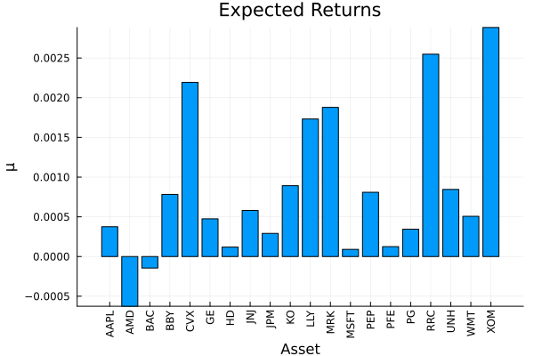
5. Linear vs logarithmic pooling
The pooling alg controls how the opinion distributions are combined.
LinearOpinionPooling(default) takes a weighted arithmetic average of the opinion probabilities. It is the "mixture of experts" rule — the consensus is a blend, so a single confident opinion can pull the mean a long way.LogarithmicOpinionPoolingtakes a weighted geometric mean (the Kullback–Leibler-optimal consensus). It is more consensus-seeking: an asset only moves far if the opinions agree, so disagreement is damped.
The two agree closely when the opinions are compatible and diverge as they conflict.
pr_lin = prior(OpinionPoolingPrior(; pes = [opinion_a, opinion_b, opinion_c],
                                   w = [0.5, 0.3, 0.2], alg = LinearOpinionPooling()), rd)
pr_log = prior(OpinionPoolingPrior(; pes = [opinion_a, opinion_b, opinion_c],
                                   w = [0.5, 0.3, 0.2], alg = LogarithmicOpinionPooling()),
               rd)

pretty_table(DataFrame(["Assets" => rd.nx, "Linear pool" => pr_lin.mu,
                        "Logarithmic pool" => pr_log.mu]); formatters = [mmtfmt],
             title = "Linear vs logarithmic pooling")
Linear vs logarithmic pooling
┌────────┬─────────────┬──────────────────┐
│ Assets │ Linear pool │ Logarithmic pool │
│ String │ Float64 │ Float64 │
├────────┼─────────────┼──────────────────┤
│ AAPL │ 0.0375 % │ 0.0367 % │
│ AMD │ -0.0626 % │ -0.0635 % │
│ BAC │ -0.0145 % │ -0.0148 % │
│ BBY │ 0.0782 % │ 0.0781 % │
│ CVX │ 0.2193 % │ 0.2193 % │
│ GE │ 0.0475 % │ 0.0475 % │
│ HD │ 0.0119 % │ 0.0114 % │
│ JNJ │ 0.058 % │ 0.0579 % │
│ JPM │ 0.0291 % │ 0.0289 % │
│ KO │ 0.0892 % │ 0.0891 % │
│ LLY │ 0.1732 % │ 0.1731 % │
│ MRK │ 0.1878 % │ 0.1878 % │
│ MSFT │ 0.0091 % │ 0.0085 % │
│ PEP │ 0.0809 % │ 0.081 % │
│ ⋮ │ ⋮ │ ⋮ │
└────────┴─────────────┴──────────────────┘
6 rows omitted6. Credibility weights and the uniform-prior fallback
The weights w say how credible each opinion is. They have a property worth knowing: if they sum to less than one, the remaining weight is assigned to the uniform prior (the unreweighted empirical distribution). So w is not just a relative split — its total is a global confidence dial. Shrinking the total pulls the consensus back toward the data and away from the views. Below we hold the relative trust fixed (5:3:2) but scale the total from 1.0 down to 0.3, watching the pooled expected returns retreat toward the empirical prior.
scales = [1.0, 0.7, 0.4]
pr_scaled = [prior(OpinionPoolingPrior(; pes = [opinion_a, opinion_b, opinion_c],
                                       w = s .* [0.5, 0.3, 0.2]), rd) for s in scales]

i_aapl = findfirst(==("AAPL"), rd.nx)
i_msft = findfirst(==("MSFT"), rd.nx)
pretty_table(DataFrame("weight total" => ["empirical (0.0)"; string.(scales)],
                       "AAPL posterior" => [pr_emp.mu[i_aapl];
                                            [p.mu[i_aapl] for p in pr_scaled]],
                       "MSFT posterior" => [pr_emp.mu[i_msft];
                                            [p.mu[i_msft] for p in pr_scaled]]);
             formatters = [mmtfmt],
             title = "Lower total weight shrinks the consensus toward the empirical prior")
Lower total weight shrinks the consensus toward the empirical prior
┌─────────────────┬────────────────┬────────────────┐
│ weight total │ AAPL posterior │ MSFT posterior │
│ String │ Float64 │ Float64 │
├─────────────────┼────────────────┼────────────────┤
│ empirical (0.0) │ -0.1126 % │ -0.1206 % │
│ 1.0 │ 0.0375 % │ 0.0091 % │
│ 0.7 │ -0.0075 % │ -0.0298 % │
│ 0.4 │ -0.0526 % │ -0.0687 % │
└─────────────────┴────────────────┴────────────────┘7. Robust pooling with p
Linear pooling trusts each opinion's weight as given. Setting p to a confidence in
pr_robust = prior(OpinionPoolingPrior(; pes = [opinion_a, opinion_b, opinion_c],
                                      w = [0.5, 0.3, 0.2], p = 0.1), rd)
A caveat from dogfooding this page: on this S&P 500 slice the robust adjustment moved the posterior mean and covariance only at the level of numerical noise (p as a lever that matters when opinions are distributionally far apart, not as a reliable knob on the consensus mean for a short single window — and reach for the credibility-weight total in section 6 when you want a dependable dial.
8. Why it matters: a consensus portfolio
Maximising the risk-adjusted ratio under the empirical prior and the pooled consensus shows how the blended views reshape the portfolio — a single allocation that honours all three opinions at once.
using Clarabel

slv = Solver(; name = :clarabel1, solver = Clarabel.Optimizer,
             settings = Dict("verbose" => false),
             check_sol = (; allow_local = true, allow_almost = true))
rf = 4.2 / 100 / 252

res_emp = optimise(MeanRisk(; obj = MaximumRatio(; rf = rf),
                            opt = JuMPOptimiser(; pe = pr_emp, slv = slv)))
res_op = optimise(MeanRisk(; obj = MaximumRatio(; rf = rf),
                           opt = JuMPOptimiser(; pe = pr_op, slv = slv)))

pretty_table(DataFrame(["Assets" => rd.nx, "Empirical" => res_emp.w,
                        "Pooled consensus" => res_op.w]); formatters = [resfmt],
             title = "Maximum-ratio weights: empirical vs pooled consensus")
Maximum-ratio weights: empirical vs pooled consensus
┌────────┬───────────┬──────────────────┐
│ Assets │ Empirical │ Pooled consensus │
│ String │ Float64 │ Float64 │
├────────┼───────────┼──────────────────┤
│ AAPL │ 0.0 % │ 0.0 % │
│ AMD │ 0.0 % │ 0.0 % │
│ BAC │ 0.0 % │ 0.0 % │
│ BBY │ 0.0 % │ 0.0 % │
│ CVX │ 0.0 % │ 0.0 % │
│ GE │ 0.0 % │ 0.0 % │
│ HD │ 0.0 % │ 0.0 % │
│ JNJ │ 0.0 % │ 0.0 % │
│ JPM │ 0.0 % │ 0.0 % │
│ KO │ 0.0 % │ 0.0 % │
│ LLY │ 0.002 % │ 2.992 % │
│ MRK │ 65.977 % │ 64.458 % │
│ MSFT │ 0.0 % │ 0.0 % │
│ PEP │ 0.0 % │ 0.0 % │
│ ⋮ │ ⋮ │ ⋮ │
└────────┴───────────┴──────────────────┘
6 rows omittedThe composition plot makes the consensus tilt visible.
plot_stacked_bar_composition([res_emp, res_op], rd; xticks = (1:2, ["Empirical", "Pooled"]))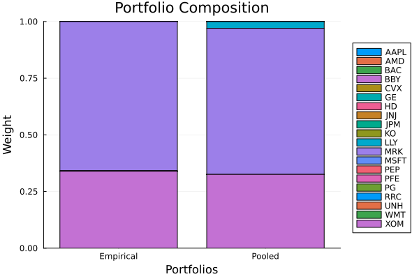
This page was generated using Literate.jl.