
The source files can be found in examples/.
Profile: factor-views desk
The fourth profile is a factor-aware desk that trades on factor views. Where the desk monthly profile expressed a thesis directly on assets ("healthcare beats energy") through entropy pooling, this desk holds its convictions in factor space — momentum will be rewarded, value will be rewarded — and lets a factor model propagate those views to every asset. It then runs the resulting posterior through a constrained optimiser, because a factor tilt left unchecked concentrates hard into whatever names load on the favoured factors.
This is the pattern that the advanced Black–Litterman page builds up variant by variant, assembled here end-to-end as a reusable book: a FactorBlackLittermanPrior, real sector constraints, and an exact allocation.
The reasoning, following the strategy decision framework:
The edge is a factor call, not a stock call — the desk has a view on factor premia, so it encodes it where it belongs and propagates it through the factor regression.
A raw factor tilt is dangerous — momentum and value concentrate, so the book is wrapped in per-asset and per-sector caps that make the tilt expressible but bounded.
Risk-adjusted, then allocated — it takes the tangency (
MaximumRatio) book on the posterior and turns it into whole shares with an exact MIP allocation.
When to reach for this
This is the template for a factor-driven book: when your conviction is about factors (momentum, value, quality, size, low-vol) rather than individual names, put the view in factor space with a factor Black–Litterman prior, then constrain the optimiser so the factor tilt diversifies into a real portfolio instead of a handful of high-loading names.
using PortfolioOptimisers, CSV, TimeSeries, DataFrames, PrettyTables, Clarabel, HiGHS,
      StatsPlots, GraphRecipes

resfmt = (v, i, j) -> begin
    return if j == 1
        v
    else
        isa(v, AbstractFloat) ? "$(round(v * 100, digits = 3)) %" : v
    end
end;
1. Data, factors, and the factor view
We load the S&P 500 slice together with its factor block (MTUM, QUAL, SIZE, USMV, VLUE), declare an asset AssetSets with sector groups (for the sector caps) and a factor AssetSets (for the views), and write the desk's thesis as factor-premia views: momentum earns 5 bps/day and value earns 3 bps/day.
X = TimeArray(CSV.File(joinpath(@__DIR__, "..", "SP500.csv.gz")); timestamp = :Date)[(end - 252):end]
F = TimeArray(CSV.File(joinpath(@__DIR__, "..", "Factors.csv.gz")); timestamp = :Date)[(end - 252):end]
rd = prices_to_returns(X, F)
prices = vec(values(X)[end, :])

asset_sets = AssetSets(;
                       dict = Dict("nx" => rd.nx, "tech" => ["AAPL", "AMD", "MSFT"],
                                   "energy" => ["CVX", "XOM", "RRC"],
                                   "healthcare" => ["JNJ", "LLY", "MRK", "PFE", "UNH"]))
factor_sets = AssetSets(; dict = Dict("nx" => rd.nf))
tau = 1 / size(rd.X, 1)

factor_views = LinearConstraintEstimator(; val = ["MTUM == 0.0005", "VLUE == 0.0003"])
LinearConstraintEstimator
val ┼ Vector{String}: ["MTUM == 0.0005", "VLUE == 0.0003"]
key ┴ nothing2. The factor Black–Litterman posterior
FactorBlackLittermanPrior takes the factor views, maps them through the asset-on-factor regression, and returns a standard asset-space posterior (mu, sigma). We keep the idiosyncratic residual variance (rsd = true) so the posterior covariance is the full asset risk, not only its factor-explained part.
prior_est = FactorBlackLittermanPrior(; pe = EmpiricalPrior(), rsd = true,
                                      sets = factor_sets, tau = tau, views = factor_views)
pr = prior(prior_est, rd)

slv = Solver(; name = :clarabel, solver = Clarabel.Optimizer,
             settings = Dict("verbose" => false),
             check_sol = (; allow_local = true, allow_almost = true))
rf = 4.2 / 100 / 2520.00016666666666666673. Why the constraints are not optional
Left unconstrained beyond a per-name cap, the tangency book on this posterior piles into the sectors that load on the favoured factors. We solve it once with only a 15% per-asset cap to see the raw tilt, then read off the sector totals.
raw = optimise(MeanRisk(; obj = MaximumRatio(; rf = rf),
                        opt = JuMPOptimiser(; pe = pr, slv = slv,
                                            wb = WeightBounds(; lb = 0.0, ub = 0.15),
                                            sets = asset_sets)))

sector_weight(w, sec) = sum(w[[findfirst(==(t), rd.nx) for t in asset_sets.dict[sec]]])
raw_sectors = DataFrame("sector" => ["tech", "energy", "healthcare"],
                        "raw tilt" => [sector_weight(raw.w, s)
                                       for s in ("tech", "energy", "healthcare")])
pretty_table(raw_sectors; formatters = [resfmt],
             title = "Sector weights with only a per-asset cap")
Sector weights with only a per-asset cap
┌────────────┬──────────┐
│ sector │ raw tilt │
│ String │ Float64 │
├────────────┼──────────┤
│ tech │ 0.0 % │
│ energy │ 35.256 % │
│ healthcare │ 44.998 % │
└────────────┴──────────┘The raw book leans heavily into healthcare and energy — the factor tilt expressed through the names that load on momentum and value on this slice. That is the conviction working, but it is also an undiversified book.
4. The constrained desk book
So the desk caps the two sectors the tilt favours — healthcare at 35% and energy at 25% — on top of the 15% per-asset bound. The factor view still drives the selection, but the caps force it to spread.
desk = optimise(MeanRisk(; obj = MaximumRatio(; rf = rf),
                         opt = JuMPOptimiser(; pe = pr, slv = slv,
                                             wb = WeightBounds(; lb = 0.0, ub = 0.15),
                                             lcse = LinearConstraintEstimator(;
                                                                              val = ["healthcare <= 0.35",
                                                                                     "energy <= 0.25"]),
                                             sets = asset_sets)))

constrained_sectors = DataFrame("sector" => ["tech", "energy", "healthcare"],
                                "constrained" => [sector_weight(desk.w, s)
                                                  for s in ("tech", "energy", "healthcare")])
pretty_table(constrained_sectors; formatters = [resfmt],
             title = "Sector weights after the 35% / 25% caps")

pretty_table(DataFrame("Asset" => rd.nx, "Weight" => desk.w); formatters = [resfmt],
             title = "Factor-views desk — constrained tangency book")
Sector weights after the 35% / 25% caps
┌────────────┬─────────────┐
│ sector │ constrained │
│ String │ Float64 │
├────────────┼─────────────┤
│ tech │ 0.0 % │
│ energy │ 25.0 % │
│ healthcare │ 35.0 % │
└────────────┴─────────────┘
Factor-views desk — constrained tangency book
┌────────┬─────────┐
│ Asset │ Weight │
│ String │ Float64 │
├────────┼─────────┤
│ AAPL │ 0.0 % │
│ AMD │ 0.0 % │
│ BAC │ 0.0 % │
│ BBY │ 0.0 % │
│ CVX │ 10.0 % │
│ GE │ 0.0 % │
│ HD │ 0.0 % │
│ JNJ │ 4.999 % │
│ JPM │ 0.0 % │
│ KO │ 15.0 % │
│ LLY │ 15.0 % │
│ MRK │ 15.0 % │
│ MSFT │ 0.0 % │
│ PEP │ 15.0 % │
│ ⋮ │ ⋮ │
└────────┴─────────┘
6 rows omittedBoth sector caps bind: healthcare comes down to 35% and energy to 25%, and the freed weight spreads into the rest of the universe. The book is still a factor-view portfolio — it just diversifies the tilt instead of betting it all on the highest-loading names.
5. Exact finite allocation
On a $1,000,000 book the desk wants the provably-best whole-share allocation, so it uses DiscreteAllocation with a MIP solver (HiGHS).
mip_slv = Solver(; name = :highs, solver = HiGHS.Optimizer,
                 settings = Dict("log_to_console" => false))
alloc = optimise(DiscreteAllocation(; slv = mip_slv),
                 FiniteAllocationInput(; w = desk.w, prices = prices, cash = 1_000_000.0))

invested = sum(alloc.shares .* prices)
pretty_table(DataFrame("Asset" => rd.nx, "Target" => desk.w,
                       "Shares" => round.(Int, alloc.shares), "Realised" => alloc.w);
             formatters = [resfmt],
             title = "\$1,000,000 allocated — invested \```math(round(Int, invested)), cash left \```(round(alloc.cash, digits = 2))")
$1,000,000 allocated — invested ```math(round(Int, invested)), cash left ```(r ⋯
┌────────┬─────────┬────────┬──────────┐
│ Asset │ Target │ Shares │ Realised │
│ String │ Float64 │ Int64 │ Float64 │
├────────┼─────────┼────────┼──────────┤
│ AAPL │ 0.0 % │ 0 │ 0.0 % │
│ AMD │ 0.0 % │ 0 │ 0.0 % │
│ BAC │ 0.0 % │ 0 │ 0.0 % │
│ BBY │ 0.0 % │ 0 │ 0.0 % │
│ CVX │ 10.0 % │ 576 │ 10.007 % │
│ GE │ 0.0 % │ 0 │ 0.0 % │
│ HD │ 0.0 % │ 0 │ 0.0 % │
│ JNJ │ 4.999 % │ 287 │ 4.996 % │
│ JPM │ 0.0 % │ 0 │ 0.0 % │
│ KO │ 15.0 % │ 2395 │ 14.995 % │
│ LLY │ 15.0 % │ 413 │ 14.996 % │
│ MRK │ 15.0 % │ 1369 │ 15.002 % │
│ MSFT │ 0.0 % │ 0 │ 0.0 % │
│ PEP │ 15.0 % │ 837 │ 15.006 % │
│ ⋮ │ ⋮ │ ⋮ │ ⋮ │
└────────┴─────────┴────────┴──────────┘
6 rows omitted6. The book
plot_stacked_bar_composition([desk], rd; xticks = (1:1, ["Factor-views desk"]))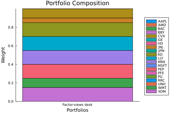
This page was generated using Literate.jl.