
The source files can be found in user_guide/.
Introduction
Welcome to the PortfolioOptimisers.jl user guide — a fast, skimmable tour of the package. Each page gives you the one minimal blessed call for a task so you can get a portfolio out the door without reading the source or the reference. It is deliberately shallow: when you want the full treatment of a topic — every variant, sweep, and trade-off — follow the cross-links into the Examples, which are deep single-topic dives.
The pipeline
PortfolioOptimisers.jl is organised as a pipeline. Data flows through a sequence of stages, and each stage is a swappable estimator:
data ─▶ moments / prior ─▶ optimiser ─▶ constraints & costs ─▶ validation ─▶ post-processingThe guide mirrors that spine, one page per stage:
Data and priors — turn prices into returns and returns into a prior (expected returns, covariance). Deep dives: moments & priors examples.
Optimisers — the breadth tour: naive, JuMP (MeanRisk, risk budgeting, near-optimal centering), clustering, and meta-optimisers. Deep dives: optimiser examples.
Constraints and costs — budgets, weight bounds, turnover, fees. Deep dives: constraints & costs examples.
Validation and tuning — cross-validation and hyperparameter search. Deep dives: validation examples.
Post-processing — discrete allocation and reporting. Deep dives: post-processing examples.
Choosing a strategy — a decision framework for picking tools by compute budget, rebalance frequency, risk appetite, and capital. Worked end-to-end profiles live in putting it together.
Reading the API
Two conventions run through the whole library. Knowing them up front makes the two-letter keyword names and the call sites read at a glance.
Abbreviations follow a scheme. Composed estimators take their sub-parts as short keyword arguments. The trailing letter tells you what kind of thing the slot holds: -e is an estimator (a configuration that still has to be run), -r is a result (an already-computed value passed downstream). So pe is a prior estimator, but a computed prior can be passed into the same slot; cle is a clustering estimator, clr a clustering result.
| Abbrev. | Slot | Abbrev. | Slot |
|---|---|---|---|
pe | prior estimator / result | slv | solver(s) |
ce | covariance estimator | me | expected-returns (mean) estimator |
ve | variance estimator | de | distance estimator |
mp | matrix-processing estimator | pdm | posdef-matrix estimator |
cle / clr | clustering estimator / result | re | regression estimator |
wb | weight bounds | opt | optimiser configuration (JuMPOptimiser / HierarchicalOptimiser) |
r | risk measure | obj | objective function |
rd | returns data (ReturnsResult) | fb | fallback estimator |
Callable signal: functor vs verb. Most stages are run with a verb applied to an estimator — prior(EmpiricalPrior(), rd), optimise(MeanRisk(…)), clusterise(…), factory(…). Risk measures are the exception: a risk measure is itself a callable functor — you call the measure value directly to evaluate the risk of a portfolio, rather than passing it to a verb. Rule of thumb: a type that names a stage (prior, optimiser, clustering) is driven by a verb; a type that names a risk quantity is called directly.
The data
Every page in the guide uses the same bundled S&P 500 slice, so the pieces compose. Loading it and glancing at the prior is the natural first step — plot_prior shows the expected returns, per-asset volatility, and correlation of the data in one view.
using PortfolioOptimisers, CSV, TimeSeries, StatsPlots, GraphRecipes

X = TimeArray(CSV.File(joinpath(@__DIR__, "../examples/SP500.csv.gz")); timestamp = :Date)[(end - 252):end]
rd = prices_to_returns(X)

plot_prior(prior(EmpiricalPrior(), rd), rd)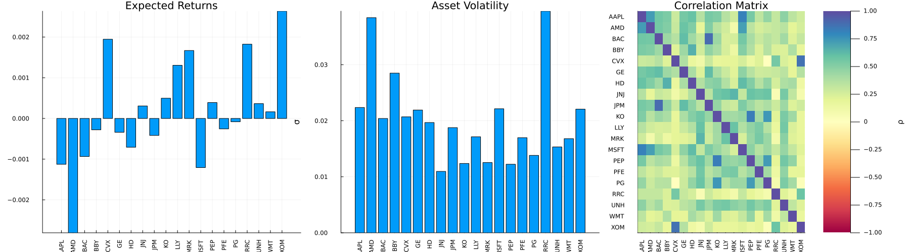
This page was generated using Literate.jl.