
The source files can be found in examples/.
Custom objectives and constraints
Every keyword on a JuMPOptimiser — bounds, budgets, turnover, fees, cardinality — is a pre-built way to shape the problem. When a mandate needs something none of them covers, PortfolioOptimisers.jl gives you two extension points that write straight against the JuMP model:
CustomJuMPObjective(thecobjkeyword) — implementadd_custom_objective_term!to price a preference, softly.CustomJuMPConstraint(theccntkeyword) — implementadd_custom_constraint!to mandate one, hard.
Each keyword takes a single estimator or a vector of them, and each hook dispatches on the estimator's type, so a term is just a struct carrying its data plus one method. Subtyping one without implementing its method is an error, not a silent no-op. This page builds both from scratch, works through the model idioms that keep them correct (the constraint scale and the homogenisation variable k), and composes several into one problem. It is the deep dive behind the one-call summary in the constraints & costs guide.
When to reach for this
Reach for a custom term when your preference is a continuous per-asset number that no group string can express — a factor score, a carbon intensity, a liquidity penalty — or a relationship between weights that isn't a plain linear bound. If it can be written as a linear/group constraint (lcse) or an existing keyword, prefer that: the built-ins are tested and composable. Custom hooks are the escape hatch, not the first tool.
using PortfolioOptimisers, CSV, TimeSeries, DataFrames, PrettyTables, Clarabel, StatsPlots,
      GraphRecipes
using JuMP: JuMP

resfmt = (v, i, j) -> begin
    return if j == 1
        v
    else
        isa(v, AbstractFloat) ? "$(round(v*100, digits=3)) %" : v
    end
end;
1. Data and a momentum score
We fix one empirical prior, a solver, and a minimum-risk baseline, so every custom term's effect is visible against the same allocation. The preference we will encode is a momentum score: each asset's trailing-63-day return, standardised across the universe. It is a continuous per-asset number — exactly the case the extension points exist for.
X = TimeArray(CSV.File(joinpath(@__DIR__, "..", "SP500.csv.gz")); timestamp = :Date)[(end - 252):end]
rd = prices_to_returns(X)
pr = prior(EmpiricalPrior(), rd)

slv = Solver(; name = :clarabel, solver = Clarabel.Optimizer,
             settings = Dict("verbose" => false),
             check_sol = (; allow_local = true, allow_almost = true))
rf = 4.2 / 100 / 252

score = let m = vec(sum(rd.X[(end - 62):end, :]; dims = 1))
    (m .- mean(m)) ./ std(m)
end

res_base = optimise(MeanRisk(; obj = MinimumRisk(),
                             opt = JuMPOptimiser(; pe = pr, slv = slv)))
MeanRiskResult
jr ┼ JuMPOptimisationResult
│ pa ┼ ProcessedJuMPOptimiserAttributes
│ │ pr ┼ LowOrderPrior
│ │ │ X ┼ 252×20 Matrix{Float64}
│ │ │ mu ┼ 20-element Vector{Float64}
│ │ │ sigma ┼ 20×20 Matrix{Float64}
│ │ │ chol ┼ nothing
│ │ │ w ┼ nothing
│ │ │ ens ┼ nothing
│ │ │ kld ┼ nothing
│ │ │ ow ┼ nothing
│ │ │ rr ┼ nothing
│ │ │ f_mu ┼ nothing
│ │ │ f_sigma ┼ nothing
│ │ │ f_w ┴ nothing
│ │ wb ┼ WeightBounds
│ │ │ lb ┼ 20-element StepRangeLen{Float64, Base.TwicePrecision{Float64}, Base.TwicePrecision{Float64}, Int64}
│ │ │ ub ┴ 20-element StepRangeLen{Float64, Base.TwicePrecision{Float64}, Base.TwicePrecision{Float64}, Int64}
│ │ lt ┼ nothing
│ │ st ┼ nothing
│ │ lcsr ┼ nothing
│ │ ctr ┼ nothing
│ │ gcardr ┼ nothing
│ │ sgcardr ┼ nothing
│ │ smtx ┼ nothing
│ │ sgmtx ┼ nothing
│ │ slt ┼ nothing
│ │ sst ┼ nothing
│ │ sglt ┼ nothing
│ │ sgst ┼ nothing
│ │ tn ┼ nothing
│ │ fees ┼ nothing
│ │ plr ┼ nothing
│ │ ret ┼ ArithmeticReturn
│ │ │ ucs ┼ nothing
│ │ │ lb ┼ nothing
│ │ │ mu ┴ 20-element Vector{Float64}
│ retcode ┼ OptimisationSuccess
│ │ res ┴ Dict{Any, Any}: Dict{Any, Any}()
│ sol ┼ JuMPOptimisationSolution
│ │ w ┴ 20-element Vector{Float64}
│ model ┼ A JuMP Model
│ │ ├ solver: Clarabel
│ │ ├ objective_sense: MIN_SENSE
│ │ │ └ objective_function_type: QuadExpr
│ │ ├ num_variables: 21
│ │ ├ num_constraints: 4
│ │ │ ├ AffExpr in MOI.EqualTo{Float64}: 1
│ │ │ ├ Vector{AffExpr} in MOI.Nonnegatives: 1
│ │ │ ├ Vector{AffExpr} in MOI.Nonpositives: 1
│ │ │ └ Vector{AffExpr} in MOI.SecondOrderCone: 1
│ │ └ Names registered in the model
│ │ └ :G, :bgt, :dev_1, :dev_1_soc, :k, :lw, :obj_expr, :ret, :risk, :risk_vec, :sc, :so, :variance_flag, :variance_risk_1, :w, :w_lb, :w_ub
fb ┴ nothingThe portfolio's momentum exposure is score' * w — the score-weighted allocation. The minimum-risk baseline does not care about momentum, so it lands wherever the risk trade-off puts it; we will push that exposure up, first softly (an objective), then hard (a constraint).
base_exposure = score' * res_base.w0.20421091836386752. A custom objective — a soft tilt
A custom objective is a struct subtyping CustomJuMPObjective, carrying whatever data the term needs, plus one method of add_custom_objective_term!. The method is handed the model mid-assembly and contributes a term to the objective penalty. Its signature is
add_custom_objective_term!(model, obj, cobj, optimiser, attrs)model— theJuMPmodel under construction.obj— theObjectiveFunctionbeing built (MinimumRisk,MaximumUtility, …). Dispatch on this if your term should differ by objective; you do not need it to get the sign right.cobj— your estimator; the argument you dispatch your method on.optimiser— the outer optimiser estimator (e.g. theMeanRiskitself). Itsoptfield is theJuMPOptimiser.attrs— theProcessedJuMPOptimiserAttributesbundle:attrs.pr(prior),attrs.ret(returns estimator),attrs.wb(bounds) and the rest of the processed problem data, if your term is data-driven rather than carrying its own numbers.
Read the weight variables with the get_w accessor rather than reaching into model[:w] — it asserts the variables have been registered and fails with a clear message if a hook runs out of order.
Contribute the term with add_to_objective_penalty! rather than touching the objective expression yourself. That single call is what makes the term correct everywhere:
The library orients your term; you just say what you mean
Some objectives are minimised and some maximised, and MaximumRatio is either depending on the risk measure — so a term written against the raw objective expression needs a sign that no single rule can supply. The penalty accumulator sidesteps this: it is folded into the objective with the factor matching whichever sense is being built, so a contribution always worsens the objective, and a reward is a negative contribution. Write -λ * something_good once and it rewards under every objective.
It also promotes an affine accumulator to a quadratic one as needed, so a quadratic term (an L2 tilt, a tracking penalty) is safe against any objective — including the affine ones, where mutating the expression directly would be a MethodError.
struct MomentumTilt{T1, T2} <: PortfolioOptimisers.CustomJuMPObjective
    score::T1
    lambda::T2
end

function PortfolioOptimisers.add_custom_objective_term!(model::JuMP.Model, obj,
                                                        cobj::MomentumTilt, optimiser,
                                                        attrs)
    w = PortfolioOptimisers.get_w(model)
    # Negative penalty == reward. No sign dispatch, no objective-type special cases.
    PortfolioOptimisers.add_to_objective_penalty!(model, -cobj.lambda * (cobj.score' * w))
    return nothing
end
lambda is the price we put on momentum relative to risk. Sweeping it traces the soft trade-off: a small lambda barely moves the book, a large one lets momentum dominate — until the term saturates and the portfolio piles into the single highest-momentum name.
lambdas = [0.0, 1e-4, 5e-4, 2e-3]
tilt_res = [optimise(MeanRisk(; obj = MinimumRisk(),
                              opt = JuMPOptimiser(; pe = pr, slv = slv,
                                                  cobj = MomentumTilt(score, l))))
            for l in lambdas]

pretty_table(DataFrame("λ (momentum price)" => lambdas,
                       "Momentum exposure" => [score' * r.w for r in tilt_res],
                       "Max weight" => [maximum(r.w) for r in tilt_res]);
             formatters = [resfmt],
             title = "A larger λ buys more momentum exposure, until it saturates")
A larger λ buys more momentum exposure, until it saturates
┌────────────────────┬───────────────────┬────────────┐
│ λ (momentum price) │ Momentum exposure │ Max weight │
│ Float64 │ Float64 │ Float64 │
├────────────────────┼───────────────────┼────────────┤
│ 0.0 │ 20.421 % │ 36.974 % │
│ 0.0001 │ 129.535 % │ 69.305 % │
│ 0.0005 │ 139.637 % │ 83.008 % │
│ 0.002 │ 139.873 % │ 88.846 % │
└────────────────────┴───────────────────┴────────────┘Note the term is homogeneous of degree one in w (it scales with the weights, just like the return and risk expressions). That is what lets it stay consistent under a ratio objective's internal rescaling — the constraint side, next, is where that rescaling needs explicit care.
3. The same term under a different sense
MaximumUtility is a maximisation, the exact opposite of the minimisation above — and the tilt needs no change at all. The identical MomentumTilt lifts its momentum exposure too, because the penalty accumulator is folded in with the factor for whichever sense is being built.
util_base = optimise(MeanRisk(; obj = MaximumUtility(),
                              opt = JuMPOptimiser(; pe = pr, slv = slv)))
util_tilt = optimise(MeanRisk(; obj = MaximumUtility(),
                              opt = JuMPOptimiser(; pe = pr, slv = slv,
                                                  cobj = MomentumTilt(score, 5e-3))))

util_exposures = (base = score' * util_base.w, tilted = score' * util_tilt.w)
(base = 1.15610715381599, tilted = 1.403239633609198)MaximumRatio needs no special case
The maximum-ratio problem is solved through a homogenising transform that, depending on the risk measure, lands the objective in either a maximisation or a risk-minimisation form — so a term written against the raw objective expression has no single correct sign. Because the contribution goes through the penalty accumulator, both forms fold it in with their own factor and the tilt rewards momentum either way. Note this fixes the sign, not the scaling: §5's k idiom still applies to any term that is not homogeneous of degree one in w.
4. A custom constraint — a hard floor
A custom constraint is the same shape: a struct subtyping CustomJuMPConstraint plus one method of add_custom_constraint!, whose signature is
add_custom_constraint!(model, ccnt, optimiser, attrs)model,optimiser,attrs— exactly as on the objective side (ccntis what you dispatch on). The two hooks take the same arguments; the objective one addsobjahead of the dispatch argument, and that is the only difference between them.
Two model idioms keep a hand-written constraint correct (see ADR 0008, JuMP model assembly): 2. Scale the constraint by get_constraint_scale (model[:sc]), so it sits on the same numerical footing as every built-in constraint.
- Multiply any constant bound by
get_k(model[:k]), the homogenisation variable. For most objectivesk == 1and this is a no-op; under a ratio objective the weights are solved in a rescaled space (w_real = w / k), and a bare constant would be compared against the rescaled weights — the wrong thing. §5 shows exactly what breaks.
struct MomentumFloor{T1, T2} <: PortfolioOptimisers.CustomJuMPConstraint
    score::T1
    floor::T2
end

function PortfolioOptimisers.add_custom_constraint!(model::JuMP.Model, ccnt::MomentumFloor,
                                                    optimiser, attrs)
    w = PortfolioOptimisers.get_w(model)
    k = PortfolioOptimisers.get_k(model)
    sc = PortfolioOptimisers.get_constraint_scale(model)
    JuMP.@constraint(model, sc * (ccnt.score' * w - ccnt.floor * k) >= 0)
    return nothing
end
Unlike the soft tilt, a floor binds exactly: the optimiser buys just enough momentum to meet it and no more, spending the rest of its freedom on risk. Sweeping the floor shows it clamping the exposure to the requested level (a floor below the baseline 0.204 simply never binds).
floors = [0.0, 0.5, 1.0, 1.35]
floor_res = [optimise(MeanRisk(; obj = MinimumRisk(),
                               opt = JuMPOptimiser(; pe = pr, slv = slv,
                                                   ccnt = MomentumFloor(score, f))))
             for f in floors]

pretty_table(DataFrame("Momentum floor" => floors,
                       "Momentum exposure" => [score' * r.w for r in floor_res],
                       "Binds?" => [score' * r.w > f + 1e-6 ? "no" : "yes"
                                    for (f, r) in zip(floors, floor_res)]);
             formatters = [resfmt], title = "A hard floor clamps the exposure to its bound")
A hard floor clamps the exposure to its bound
┌────────────────┬───────────────────┬────────┐
│ Momentum floor │ Momentum exposure │ Binds? │
│ Float64 │ Float64 │ String │
├────────────────┼───────────────────┼────────┤
│ 0.0 │ 20.436 % │ no │
│ 0.5 │ 50.0 % │ no │
│ 1.0 │ 100.0 % │ yes │
│ 1.35 │ 135.0 % │ yes │
└────────────────┴───────────────────┴────────┘5. Why the k idiom matters
To see idiom (2) pay off, here is the same floor written without the * k — the mistake most people make first, because it is invisible under MinimumRisk (where k == 1).
struct MomentumFloorNoK{T1, T2} <: PortfolioOptimisers.CustomJuMPConstraint
    score::T1
    floor::T2
end
function PortfolioOptimisers.add_custom_constraint!(model::JuMP.Model,
                                                    ccnt::MomentumFloorNoK, opt, attrs)
    w = PortfolioOptimisers.get_w(model)
    sc = PortfolioOptimisers.get_constraint_scale(model)
    JuMP.@constraint(model, sc * (ccnt.score' * w - ccnt.floor) >= 0)  # forgot `* k`
    return nothing
end
Under MaximumRatio the homogenisation variable k is a genuine free variable, so the two versions diverge. The correct floor binds the recovered exposure exactly at the bound; the k-less one binds it at some fixed level of the rescaled weights — which, at floor = 1.38, lands below the requested floor, silently breaking the mandate.
k_floors = [1.30, 1.35, 1.38]
k_compare = [(f,
              score' * optimise(MeanRisk(; obj = MaximumRatio(; rf = rf),
                            opt = JuMPOptimiser(; pe = pr, slv = slv,
                                                ccnt = MomentumFloor(score, f)))).w,
              score' * optimise(MeanRisk(; obj = MaximumRatio(; rf = rf),
                            opt = JuMPOptimiser(; pe = pr, slv = slv,
                                                ccnt = MomentumFloorNoK(score, f)))).w)
             for f in k_floors]

pretty_table(DataFrame("Requested floor" => first.(k_compare),
                       "With * k (correct)" => getindex.(k_compare, 2),
                       "Without * k (wrong)" => getindex.(k_compare, 3));
             formatters = [resfmt],
             title = "Under a ratio objective, only the k-scaled floor binds where asked")
Under a ratio objective, only the k-scaled floor binds where asked
┌─────────────────┬────────────────────┬─────────────────────┐
│ Requested floor │ With * k (correct) │ Without * k (wrong) │
│ Float64 │ Float64 │ Float64 │
├─────────────────┼────────────────────┼─────────────────────┤
│ 1.3 │ 130.0 % │ 136.853 % │
│ 1.35 │ 135.0 % │ 136.933 % │
│ 1.38 │ 138.0 % │ 136.983 % │
└─────────────────┴────────────────────┴─────────────────────┘6. Composing several custom pieces
Both keywords accept a vector of estimators, applied in order — the hooks iterate and dispatch each element. That is how you stack custom terms without folding them into one struct.
A band from two constraints. Pair the floor with its mirror image — a cap, the same idiom with the inequality flipped — and the two together bound the exposure into a corridor. Define the cap first (as always, every custom type before the optimiser that uses it):
struct MomentumCap{T1, T2} <: PortfolioOptimisers.CustomJuMPConstraint
    score::T1
    cap::T2
end
function PortfolioOptimisers.add_custom_constraint!(model::JuMP.Model, ccnt::MomentumCap,
                                                    optimiser, attrs)
    w = PortfolioOptimisers.get_w(model)
    k = PortfolioOptimisers.get_k(model)
    sc = PortfolioOptimisers.get_constraint_scale(model)
    JuMP.@constraint(model, sc * (ccnt.cap * k - ccnt.score' * w) >= 0)
    return nothing
end

band = optimise(MeanRisk(; obj = MinimumRisk(),
                         opt = JuMPOptimiser(; pe = pr, slv = slv,
                                             ccnt = [MomentumFloor(score, 0.5),
                                                     MomentumCap(score, 0.8)])))
MeanRiskResult
jr ┼ JuMPOptimisationResult
│ pa ┼ ProcessedJuMPOptimiserAttributes
│ │ pr ┼ LowOrderPrior
│ │ │ X ┼ 252×20 Matrix{Float64}
│ │ │ mu ┼ 20-element Vector{Float64}
│ │ │ sigma ┼ 20×20 Matrix{Float64}
│ │ │ chol ┼ nothing
│ │ │ w ┼ nothing
│ │ │ ens ┼ nothing
│ │ │ kld ┼ nothing
│ │ │ ow ┼ nothing
│ │ │ rr ┼ nothing
│ │ │ f_mu ┼ nothing
│ │ │ f_sigma ┼ nothing
│ │ │ f_w ┴ nothing
│ │ wb ┼ WeightBounds
│ │ │ lb ┼ 20-element StepRangeLen{Float64, Base.TwicePrecision{Float64}, Base.TwicePrecision{Float64}, Int64}
│ │ │ ub ┴ 20-element StepRangeLen{Float64, Base.TwicePrecision{Float64}, Base.TwicePrecision{Float64}, Int64}
│ │ lt ┼ nothing
│ │ st ┼ nothing
│ │ lcsr ┼ nothing
│ │ ctr ┼ nothing
│ │ gcardr ┼ nothing
│ │ sgcardr ┼ nothing
│ │ smtx ┼ nothing
│ │ sgmtx ┼ nothing
│ │ slt ┼ nothing
│ │ sst ┼ nothing
│ │ sglt ┼ nothing
│ │ sgst ┼ nothing
│ │ tn ┼ nothing
│ │ fees ┼ nothing
│ │ plr ┼ nothing
│ │ ret ┼ ArithmeticReturn
│ │ │ ucs ┼ nothing
│ │ │ lb ┼ nothing
│ │ │ mu ┴ 20-element Vector{Float64}
│ retcode ┼ OptimisationSuccess
│ │ res ┴ Dict{Any, Any}: Dict{Any, Any}()
│ sol ┼ JuMPOptimisationSolution
│ │ w ┴ 20-element Vector{Float64}
│ model ┼ A JuMP Model
│ │ ├ solver: Clarabel
│ │ ├ objective_sense: MIN_SENSE
│ │ │ └ objective_function_type: QuadExpr
│ │ ├ num_variables: 21
│ │ ├ num_constraints: 6
│ │ │ ├ AffExpr in MOI.EqualTo{Float64}: 1
│ │ │ ├ AffExpr in MOI.GreaterThan{Float64}: 2
│ │ │ ├ Vector{AffExpr} in MOI.Nonnegatives: 1
│ │ │ ├ Vector{AffExpr} in MOI.Nonpositives: 1
│ │ │ └ Vector{AffExpr} in MOI.SecondOrderCone: 1
│ │ └ Names registered in the model
│ │ └ :G, :bgt, :dev_1, :dev_1_soc, :k, :lw, :obj_expr, :ret, :risk, :risk_vec, :sc, :so, :variance_flag, :variance_risk_1, :w, :w_lb, :w_ub
fb ┴ nothingAdditive objectives. A cobj vector contributes each term to the same penalty accumulator, so two 1e-4 tilts compose into one of strength 2e-4 — a quick sanity check that vectors accumulate rather than replace:
two_tilts = optimise(MeanRisk(; obj = MinimumRisk(),
                              opt = JuMPOptimiser(; pe = pr, slv = slv,
                                                  cobj = [MomentumTilt(score, 1e-4),
                                                          MomentumTilt(score, 1e-4)])))
one_double = optimise(MeanRisk(; obj = MinimumRisk(),
                               opt = JuMPOptimiser(; pe = pr, slv = slv,
                                                   cobj = MomentumTilt(score, 2e-4))))

composition = (band = score' * band.w, two_1e4_tilts = score' * two_tilts.w,
               one_2e4_tilt = score' * one_double.w)
(band = 0.5000014186440694, two_1e4_tilts = 1.3694760110199082, one_2e4_tilt = 1.3694760110199082)The band sits inside [0.5, 0.8], and the two stacked tilts land on exactly the same exposure as the single double-strength tilt — vectors compose.
Objective and constraint together. Nothing stops you mixing them: a soft tilt and a hard floor in the same problem, each through its own keyword.
res_both = optimise(MeanRisk(; obj = MinimumRisk(),
                             opt = JuMPOptimiser(; pe = pr, slv = slv,
                                                 cobj = MomentumTilt(score, 1e-4),
                                                 ccnt = MomentumFloor(score, 1.0))))
MeanRiskResult
jr ┼ JuMPOptimisationResult
│ pa ┼ ProcessedJuMPOptimiserAttributes
│ │ pr ┼ LowOrderPrior
│ │ │ X ┼ 252×20 Matrix{Float64}
│ │ │ mu ┼ 20-element Vector{Float64}
│ │ │ sigma ┼ 20×20 Matrix{Float64}
│ │ │ chol ┼ nothing
│ │ │ w ┼ nothing
│ │ │ ens ┼ nothing
│ │ │ kld ┼ nothing
│ │ │ ow ┼ nothing
│ │ │ rr ┼ nothing
│ │ │ f_mu ┼ nothing
│ │ │ f_sigma ┼ nothing
│ │ │ f_w ┴ nothing
│ │ wb ┼ WeightBounds
│ │ │ lb ┼ 20-element StepRangeLen{Float64, Base.TwicePrecision{Float64}, Base.TwicePrecision{Float64}, Int64}
│ │ │ ub ┴ 20-element StepRangeLen{Float64, Base.TwicePrecision{Float64}, Base.TwicePrecision{Float64}, Int64}
│ │ lt ┼ nothing
│ │ st ┼ nothing
│ │ lcsr ┼ nothing
│ │ ctr ┼ nothing
│ │ gcardr ┼ nothing
│ │ sgcardr ┼ nothing
│ │ smtx ┼ nothing
│ │ sgmtx ┼ nothing
│ │ slt ┼ nothing
│ │ sst ┼ nothing
│ │ sglt ┼ nothing
│ │ sgst ┼ nothing
│ │ tn ┼ nothing
│ │ fees ┼ nothing
│ │ plr ┼ nothing
│ │ ret ┼ ArithmeticReturn
│ │ │ ucs ┼ nothing
│ │ │ lb ┼ nothing
│ │ │ mu ┴ 20-element Vector{Float64}
│ retcode ┼ OptimisationSuccess
│ │ res ┴ Dict{Any, Any}: Dict{Any, Any}()
│ sol ┼ JuMPOptimisationSolution
│ │ w ┴ 20-element Vector{Float64}
│ model ┼ A JuMP Model
│ │ ├ solver: Clarabel
│ │ ├ objective_sense: MIN_SENSE
│ │ │ └ objective_function_type: QuadExpr
│ │ ├ num_variables: 21
│ │ ├ num_constraints: 5
│ │ │ ├ AffExpr in MOI.EqualTo{Float64}: 1
│ │ │ ├ AffExpr in MOI.GreaterThan{Float64}: 1
│ │ │ ├ Vector{AffExpr} in MOI.Nonnegatives: 1
│ │ │ ├ Vector{AffExpr} in MOI.Nonpositives: 1
│ │ │ └ Vector{AffExpr} in MOI.SecondOrderCone: 1
│ │ └ Names registered in the model
│ │ └ :G, :bgt, :dev_1, :dev_1_soc, :k, :lw, :obj_expr, :op, :ret, :risk, :risk_vec, :sc, :so, :variance_flag, :variance_risk_1, :w, :w_lb, :w_ub
fb ┴ nothing7. Comparing the effect
Same prior, same minimum-risk objective — only the custom term changes the allocation. The soft tilt leans toward momentum as far as the risk trade-off allows; the hard floor and the band pin the exposure to a level; combining them does both.
results = [res_base, tilt_res[2], floor_res[3], band, res_both]
labels = ["Base", "Tilt λ=1e-4", "Floor 1.0", "Band [0.5,0.8]", "Tilt + floor"]

pretty_table(DataFrame(["Asset" => rd.nx,
                        [labels[i] => results[i].w for i in eachindex(results)]...]);
             formatters = [resfmt], title = "Weights under each custom term")

plot_stacked_bar_composition(results, rd; xticks = (1:length(labels), labels))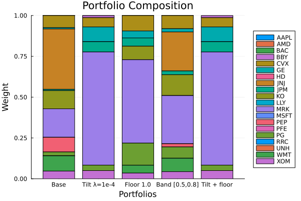
This page was generated using Literate.jl.