The source files can be found in examples/.
Budget constraints
The budget is the sum of the portfolio weights. The short budget is the absolute value of the sum of the negative weights.
The two constraints act on different variables. The budget constraint acts on the weights. The short budget constraint acts on one relaxation variable per asset, and each relaxation variable must be at least the absolute value of that asset's negative weight. The solver is free to set a relaxation variable above that value. Then the short positions you print can sum to less than the short budget, and the constraint is still met. The short budget is therefore an upper bound on the short positions. Set xbgt = true on the JuMPOptimiser to make it exact, which turns the problem into a mixed-integer one.
using PortfolioOptimisers, PrettyTablestsfmt = (v, i, j) -> begin if j == 1 return Date(v) else return v endend;resfmt = (v, i, j) -> begin if j == 1 return v else return isa(v, Number) ? "$(round(v*100, digits=3)) %" : v endend;mipresfmt = (v, i, j) -> begin if j ∈ (1, 2, 3) return v else return isa(v, Number) ? "$(round(v*100, digits=3)) %" : v endend;1. Data
We use one year of daily prices of 20 assets of the S&P 500, and convert them to returns.
using CSV, TimeSeries, DataFramesX = TimeArray(CSV.File(joinpath(@__DIR__, "..", "SP500.csv.gz")); timestamp = :Date)[(end - 252):end]pretty_table(X[(end - 5):end]; formatters = [tsfmt])rd = prices_to_returns(X)ReturnsResult
nx ┼ 20-element Vector{String}
X ┼ 252×20 Matrix{Float64}
nf ┼ nothing
F ┼ nothing
nb ┼ nothing
B ┼ nothing
ne ┼ nothing
E ┼ nothing
ts ┼ 252-element Vector{Date}
iv ┼ nothing
ivpa ┼ nothing
pnl ┴ nothing
2. Solvers, risk measure and prior
We give the optimiser a vector of four Clarabel settings. If one fails to solve a problem, the optimiser tries the next. The discrete allocation needs a mixed-integer solver, and one HiGHS instance is enough.
using Clarabel, HiGHSslv = [Solver(; name = :clarabel1, solver = Clarabel.Optimizer, settings = Dict("verbose" => false), check_sol = (; allow_local = true, allow_almost = true)), Solver(; name = :clarabel3, solver = Clarabel.Optimizer, settings = Dict("verbose" => false, "max_step_fraction" => 0.9), check_sol = (; allow_local = true, allow_almost = true)), Solver(; name = :clarabel5, solver = Clarabel.Optimizer, settings = Dict("verbose" => false, "max_step_fraction" => 0.8), check_sol = (; allow_local = true, allow_almost = true)), Solver(; name = :clarabel7, solver = Clarabel.Optimizer, settings = Dict("verbose" => false, "max_step_fraction" => 0.70), check_sol = (; allow_local = true, allow_almost = true))];mip_slv = Solver(; name = :highs1, solver = HiGHS.Optimizer, settings = Dict("log_to_console" => false), check_sol = (; allow_local = true, allow_almost = true));We minimise the EntropicValueatRisk, and we compute the prior once so that every optimisation below reuses it.
r = EntropicValueatRisk()pr = prior(EmpiricalPrior(), rd)LowOrderPrior
X ┼ 252×20 Matrix{Float64}
o_X ┼ nothing
mu ┼ 20-element Vector{Float64}
sigma ┼ 20×20 Matrix{Float64}
chol ┼ nothing
w ┼ nothing
ens ┼ nothing
eoc ┼ Tuple{Nothing, Nothing}: (nothing, nothing)
kld ┼ nothing
ow ┼ nothing
rr ┼ nothing
fpr ┼ nothing
x_src ┼ nothing
ss_gaps ┼ nothing
pc ┴ nothing
3. Exact budget constraints
An exact budget fixes the sum of the weights at one number. For each portfolio we also allocate a finite amount of cash, to show what the budget means in shares and currency.
3.1 Portfolios with an exact budget
3.1.1 Fully invested long-only portfolio
We start with the default, bgt = 1. The weights sum to one, so the portfolio is fully invested.
opt1 = JuMPOptimiser(; pe = pr, slv = slv)mr1 = MeanRisk(; r = r, opt = opt1)MeanRisk
opt ┼ JuMPOptimiser
│ pe ┼ LowOrderPrior
│ │ X ┼ 252×20 Matrix{Float64}
│ │ o_X ┼ nothing
│ │ mu ┼ 20-element Vector{Float64}
│ │ sigma ┼ 20×20 Matrix{Float64}
│ │ chol ┼ nothing
│ │ w ┼ nothing
│ │ ens ┼ nothing
│ │ eoc ┼ Tuple{Nothing, Nothing}: (nothing, nothing)
│ │ kld ┼ nothing
│ │ ow ┼ nothing
│ │ rr ┼ nothing
│ │ fpr ┼ nothing
│ │ x_src ┼ nothing
│ │ ss_gaps ┼ nothing
│ │ pc ┴ nothing
│ slv ┼ 4-element Vector{Solver}
│ │ Solver ⋯
│ │ Solver ⋯
│ │ Solver ⋯
│ │ Solver ⋯
│ cbe ┼ ConstraintBlock
│ │ wb ┼ WeightBounds
│ │ │ lb ┼ Float64: 0.0
│ │ │ ub ┴ Float64: 1.0
│ │ sbgt ┼ nothing
│ │ gbgt ┼ nothing
│ │ lt ┼ nothing
│ │ st ┼ nothing
│ │ lcse ┼ nothing
│ │ cte ┼ nothing
│ │ gcarde ┼ nothing
│ │ sgcarde ┼ nothing
│ │ smtx ┼ nothing
│ │ sgmtx ┼ nothing
│ │ slt ┼ nothing
│ │ sst ┼ nothing
│ │ sglt ┼ nothing
│ │ sgst ┼ nothing
│ │ tn ┼ nothing
│ │ sets ┼ nothing
│ │ tr ┼ nothing
│ │ ple ┼ nothing
│ │ ccnt ┼ nothing
│ │ cobj ┼ nothing
│ │ ss ┼ nothing
│ │ card ┼ nothing
│ │ scard ┼ nothing
│ │ l2c ┼ nothing
│ │ lpc ┼ nothing
│ │ linfc ┼ nothing
│ │ l1 ┼ nothing
│ │ l2 ┼ nothing
│ │ lp ┼ nothing
│ │ linf ┼ nothing
│ │ xbgt ┴ Bool: false
│ bgt ┼ Float64: 1.0
│ fees ┼ nothing
│ ret ┼ ArithmeticReturn
│ │ settings ┼ JuMPReturnsSettings
│ │ │ scale ┼ Float64: 1.0
│ │ │ lb ┼ nothing
│ │ │ rte ┼ Bool: true
│ │ │ fee ┼ Bool: true
│ │ │ mic ┴ Bool: true
│ │ ucs ┼ nothing
│ │ mu ┼ nothing
│ │ mtx_sqrt ┴ EigenFallbackSquareRoot()
│ sca ┼ nothing
│ sc ┼ Int64: 1
│ so ┼ Int64: 1
│ strict ┴ Bool: false
r ┼ EntropicValueatRisk
│ settings ┼ RiskMeasureSettings
│ │ scale ┼ Float64: 1.0
│ │ ub ┼ nothing
│ │ rke ┴ Bool: true
│ slv ┼ nothing
│ alpha ┼ Float64: 0.05
│ w ┴ nothing
obj ┼ MinimumRisk()
wi ┼ nothing
fb ┴ nothing
The printed estimator shows the defaults. wb is a WeightBounds with a lower bound lb = 0.0 and an upper bound ub = 1.0 on each weight, and the budget is bgt = 1.0.
We optimise, then print the budget and the long and short budgets. The last line is true when every weight is inside its bounds.
res1 = optimise(mr1)println("budget: $(sum(res1.w))")println("long budget: $(sum(res1.w[res1.w .>= zero(eltype(res1.w))]))")println("short budget: $(sum(res1.w[res1.w .< zero(eltype(res1.w))]))")println("weight bounds: $(all(x -> zero(x) <= x <= one(x), res1.w))")budget: 0.9999999998112571
long budget: 0.9999999998112571
short budget: 0.0
weight bounds: trueWe allocate 4206.9 units of cash to this portfolio with a DiscreteAllocation, which buys whole shares at the last prices.
da = DiscreteAllocation(; slv = mip_slv)mip_res1 = optimise(da, FiniteAllocationInput(; w = res1.w, prices = vec(values(X[end])), cash = 4206.9))pretty_table(DataFrame(:assets => rd.nx, :shares => mip_res1.shares, :cost => mip_res1.cost, :opt_weights => res1.w, :mip_weights => mip_res1.w); formatters = [mipresfmt])println("long cost + short cost = cost = $(sum(mip_res1.cost))")println("long cost: $(sum(mip_res1.cost[mip_res1.cost .>= zero(eltype(mip_res1.cost))]))")println("short cost: $(sum(mip_res1.cost[mip_res1.cost .< zero(eltype(mip_res1.cost))]))")println("remaining cash: $(mip_res1.cash)")println("used cash ≈ available cash: $(isapprox(sum(mip_res1.cost) + mip_res1.cash, 4206.9))")┌────────┬─────────┬─────────┬─────────────┬─────────────┐
│ assets │ shares │ cost │ opt_weights │ mip_weights │
│ String │ Float64 │ Float64 │ Float64 │ Float64 │
├────────┼─────────┼─────────┼─────────────┼─────────────┤
│ AAPL │ 0.0 │ 0.0 │ 0.0 % │ 0.0 % │
│ AMD │ 0.0 │ 0.0 │ 0.0 % │ 0.0 % │
│ BAC │ 1.0 │ 32.301 │ 0.0 % │ 0.768 % │
│ BBY │ 0.0 │ 0.0 │ 0.0 % │ 0.0 % │
│ CVX │ 5.0 │ 868.64 │ 21.386 % │ 20.655 % │
│ GE │ 0.0 │ 0.0 │ 0.0 % │ 0.0 % │
│ HD │ 0.0 │ 0.0 │ 0.0 % │ 0.0 % │
│ JNJ │ 13.0 │ 2263.11 │ 55.414 % │ 53.815 % │
│ JPM │ 0.0 │ 0.0 │ 0.0 % │ 0.0 % │
│ KO │ 0.0 │ 0.0 │ 0.0 % │ 0.0 % │
│ LLY │ 0.0 │ 0.0 │ 0.0 % │ 0.0 % │
│ MRK │ 8.0 │ 876.648 │ 21.207 % │ 20.846 % │
│ MSFT │ 0.0 │ 0.0 │ 0.0 % │ 0.0 % │
│ PEP │ 0.0 │ 0.0 │ 0.0 % │ 0.0 % │
│ PFE │ 0.0 │ 0.0 │ 0.0 % │ 0.0 % │
│ PG │ 0.0 │ 0.0 │ 0.0 % │ 0.0 % │
│ RRC │ 1.0 │ 24.497 │ 0.0 % │ 0.583 % │
│ UNH │ 0.0 │ 0.0 │ 0.0 % │ 0.0 % │
│ WMT │ 1.0 │ 140.181 │ 1.993 % │ 3.333 % │
│ XOM │ 0.0 │ 0.0 │ 0.0 % │ 0.0 % │
└────────┴─────────┴─────────┴─────────────┴─────────────┘
long cost + short cost = cost = 4205.372
long cost: 4205.372
short cost: 0.0
remaining cash: 1.5279999999993379
used cash ≈ available cash: true3.1.2 Market neutral portfolio with the maximum ratio of return to risk
A market neutral portfolio has weights that sum to zero, so its budget is zero and its long and short positions are equal in size. To get weights that are not all zero, it needs a short budget above zero and lower weight bounds below zero.
You give the short budget as a positive number. We set the weight bounds to -1 and 1, the short budget to 1 and the budget to 0. The long positions then sum to at most 1, and the short positions to at most 1 in size.
With a budget of zero, the minimum risk portfolio is all zeros, because zero weights meet every constraint and have no risk. We maximise the ratio of return to risk instead.
rf = 4.2 / 100 / 252opt2 = JuMPOptimiser(; pe = pr, slv = slv, bgt = 0, sbgt = 1, wb = WeightBounds(; lb = -1.0, ub = 1.0))mr2 = MeanRisk(; r = r, obj = MaximumRatio(; rf = rf), opt = opt2)res2 = optimise(mr2)println("budget: $(sum(res2.w))")println("long budget: $(sum(res2.w[res2.w .>= zero(eltype(res2.w))]))")println("short budget: $(sum(res2.w[res2.w .< zero(eltype(res2.w))]))")println("weight bounds: $(all(x -> -one(x) <= x <= one(x), res2.w))")budget: -2.953180370602118e-17
long budget: 0.9999936023635555
short budget: -0.9999936023635557
weight bounds: trueWe allocate the same cash. If the portfolio uses its whole short budget, the long cost and the short cost are each close to 4206.9 in size, and their sum is close to zero. The allocation buys whole shares, and the costs differ from those numbers by the price of less than one share of each asset.
The discrete allocation splits the cash between the long and the short positions from the weights, so you do not split it yourself. By default the short sales pay for the long positions, which is what ProceedsCollateral states. The proceeds of the short sales stay in the account, so the remaining cash is close to the cash. The last line is true when the costs plus the remaining cash equal the cash. CashCollateral is the other rule: the short sales give no cash, and the long and short costs together stay within the cash.
mip_res2 = optimise(da, FiniteAllocationInput(; w = res2.w, prices = vec(values(X[end])), cash = 4206.9))pretty_table(DataFrame(:assets => rd.nx, :shares => mip_res2.shares, :cost => mip_res2.cost, :opt_weights => res2.w, :mip_weights => mip_res2.w); formatters = [mipresfmt])println("long cost + short cost = cost = $(sum(mip_res2.cost))")println("long cost: $(sum(mip_res2.cost[mip_res2.cost .>= zero(eltype(mip_res2.cost))]))")println("short cost: $(sum(mip_res2.cost[mip_res2.cost .< zero(eltype(mip_res2.cost))]))")println("remaining cash: $(mip_res2.cash)")println("used cash ≈ available cash: $(isapprox(sum(mip_res2.cost) + mip_res2.cash, 4206.9))")┌────────┬─────────┬──────────┬─────────────┬─────────────┐
│ assets │ shares │ cost │ opt_weights │ mip_weights │
│ String │ Float64 │ Float64 │ Float64 │ Float64 │
├────────┼─────────┼──────────┼─────────────┼─────────────┤
│ AAPL │ -1.0 │ -125.674 │ -2.526 % │ -2.999 % │
│ AMD │ -2.0 │ -125.14 │ -3.226 % │ -2.986 % │
│ BAC │ -21.0 │ -678.321 │ -16.732 % │ -16.188 % │
│ BBY │ 1.0 │ 78.279 │ 0.837 % │ 1.895 % │
│ CVX │ 0.0 │ 0.0 │ 0.001 % │ 0.0 % │
│ GE │ 6.0 │ 383.298 │ 8.532 % │ 9.281 % │
│ HD │ 0.0 │ -0.0 │ -3.235 % │ -0.0 % │
│ JNJ │ -4.0 │ -696.34 │ -17.975 % │ -16.618 % │
│ JPM │ 3.0 │ 388.725 │ 8.859 % │ 9.412 % │
│ KO │ 23.0 │ 1440.01 │ 33.949 % │ 34.867 % │
│ LLY │ 0.0 │ 0.0 │ 3.536 % │ 0.0 % │
│ MRK │ 15.0 │ 1643.72 │ 39.716 % │ 39.799 % │
│ MSFT │ -1.0 │ -233.434 │ -7.632 % │ -5.571 % │
│ PEP │ -6.0 │ -1075.67 │ -26.22 % │ -25.671 % │
│ PFE │ -12.0 │ -591.0 │ -13.952 % │ -14.104 % │
│ PG │ 0.0 │ -0.0 │ -0.0 % │ -0.0 % │
│ RRC │ 8.0 │ 195.976 │ 4.572 % │ 4.745 % │
│ UNH │ -1.0 │ -524.422 │ -7.253 % │ -12.515 % │
│ WMT │ -1.0 │ -140.181 │ -1.248 % │ -3.345 % │
│ XOM │ 0.0 │ 0.0 │ 0.0 % │ 0.0 % │
└────────┴─────────┴──────────┴─────────────┴─────────────┘
long cost + short cost = cost = -60.17999999999981
long cost: 4130.0
short cost: -4190.179999999999
remaining cash: 4267.079999999998
used cash ≈ available cash: true3.1.3 Short-only portfolio
We now make a short-only portfolio, with a budget of -1 and weights between -1 and 0.
opt3 = JuMPOptimiser(; pe = pr, slv = slv, bgt = -1, sbgt = 1, wb = WeightBounds(; lb = -1.0, ub = 0.0))mr3 = MeanRisk(; r = r, obj = MinimumRisk(), opt = opt3)res3 = optimise(mr3)println("budget: $(sum(res3.w))")println("long budget: $(sum(res3.w[res3.w .>= zero(eltype(res3.w))]))")println("short budget: $(sum(res3.w[res3.w .< zero(eltype(res3.w))]))")println("weight bounds: $(all(x -> -one(x) <= x <= zero(x), res3.w))")budget: -0.9999999995925793
long budget: 0.0
short budget: -0.9999999995925793
weight bounds: trueWe allocate the same cash to the short-only portfolio. The proceeds of the short sales stay in the account beside the cash, so the remaining cash is close to twice the cash. The last line is true when the costs plus the remaining cash equal the cash.
mip_res3 = optimise(da, FiniteAllocationInput(; w = res3.w, prices = vec(values(X[end])), cash = 4206.9))pretty_table(DataFrame(:assets => rd.nx, :shares => mip_res3.shares, :cost => mip_res3.cost, :opt_weights => res3.w, :mip_weights => mip_res3.w); formatters = [mipresfmt])println("long cost + short cost = cost = $(sum(mip_res3.cost))")println("long cost: $(sum(mip_res3.cost[mip_res3.cost .>= zero(eltype(mip_res3.cost))]))")println("short cost: $(sum(mip_res3.cost[mip_res3.cost .< zero(eltype(mip_res3.cost))]))")println("remaining cash: $(mip_res3.cash)")println("used cash ≈ available cash: $(isapprox(sum(mip_res3.cost) + mip_res3.cash, 4206.9))")┌────────┬─────────┬──────────┬─────────────┬─────────────┐
│ assets │ shares │ cost │ opt_weights │ mip_weights │
│ String │ Float64 │ Float64 │ Float64 │ Float64 │
├────────┼─────────┼──────────┼─────────────┼─────────────┤
│ AAPL │ 0.0 │ -0.0 │ -0.0 % │ -0.0 % │
│ AMD │ 0.0 │ -0.0 │ -0.0 % │ -0.0 % │
│ BAC │ -1.0 │ -32.301 │ -0.0 % │ -0.768 % │
│ BBY │ 0.0 │ -0.0 │ -0.0 % │ -0.0 % │
│ CVX │ 0.0 │ -0.0 │ -0.0 % │ -0.0 % │
│ GE │ -3.0 │ -191.649 │ -4.404 % │ -4.558 % │
│ HD │ -1.0 │ -311.22 │ -5.068 % │ -7.401 % │
│ JNJ │ -2.0 │ -348.17 │ -9.44 % │ -8.28 % │
│ JPM │ 0.0 │ -0.0 │ -0.0 % │ -0.0 % │
│ KO │ 0.0 │ -0.0 │ -0.0 % │ -0.0 % │
│ LLY │ 0.0 │ -0.0 │ -4.646 % │ -0.0 % │
│ MRK │ -1.0 │ -109.581 │ -3.636 % │ -2.606 % │
│ MSFT │ 0.0 │ -0.0 │ -0.0 % │ -0.0 % │
│ PEP │ -8.0 │ -1434.22 │ -31.89 % │ -34.108 % │
│ PFE │ -7.0 │ -344.75 │ -7.611 % │ -8.199 % │
│ PG │ 0.0 │ -0.0 │ -0.0 % │ -0.0 % │
│ RRC │ -7.0 │ -171.479 │ -3.988 % │ -4.078 % │
│ UNH │ 0.0 │ -0.0 │ -0.0 % │ -0.0 % │
│ WMT │ -9.0 │ -1261.63 │ -29.317 % │ -30.003 % │
│ XOM │ 0.0 │ -0.0 │ -0.0 % │ -0.0 % │
└────────┴─────────┴──────────┴─────────────┴─────────────┘
long cost + short cost = cost = -4205.003000000001
long cost: -0.0
short cost: -4205.003
remaining cash: 8411.903
used cash ≈ available cash: true3.1.4 Leveraged portfolios
A budget above one gives a leveraged portfolio. We set bgt = 1.3 on a long-only portfolio, so the weights sum to 1.3.
opt4 = JuMPOptimiser(; pe = pr, slv = slv, bgt = 1.3)mr4 = MeanRisk(; r = r, opt = opt4)res4 = optimise(mr4)println("budget: $(sum(res4.w))")println("long budget: $(sum(res4.w[res4.w .>= zero(eltype(res4.w))]))")println("short budget: $(sum(res4.w[res4.w .< zero(eltype(res4.w))]))")println("weight bounds: $(all(x -> zero(x) <= x <= one(x), res4.w))")budget: 1.299999999782898
long budget: 1.299999999782898
short budget: 0.0
weight bounds: trueWe allocate the same cash. The costs sum to about 1.3 times the cash, because the budget is 1.3. The portfolio borrows 0.3 times the cash, so the remaining cash is negative, and the costs plus the remaining cash equal the cash.
mip_res4 = optimise(da, FiniteAllocationInput(; w = res4.w, prices = vec(values(X[end])), cash = 4206.9))pretty_table(DataFrame(:assets => rd.nx, :shares => mip_res4.shares, :cost => mip_res4.cost, :opt_weights => res4.w, :mip_weights => mip_res4.w); formatters = [mipresfmt])println("long cost + short cost = cost = $(sum(mip_res4.cost))")println("long cost: $(sum(mip_res4.cost[mip_res4.cost .>= zero(eltype(mip_res4.cost))]))")println("short cost: $(sum(mip_res4.cost[mip_res4.cost .< zero(eltype(mip_res4.cost))]))")println("remaining cash: $(mip_res4.cash)")println("used cash ≈ available cash: $(isapprox(sum(mip_res4.cost) + mip_res4.cash, 4206.9))")┌────────┬─────────┬─────────┬─────────────┬─────────────┐
│ assets │ shares │ cost │ opt_weights │ mip_weights │
│ String │ Float64 │ Float64 │ Float64 │ Float64 │
├────────┼─────────┼─────────┼─────────────┼─────────────┤
│ AAPL │ 0.0 │ 0.0 │ 0.0 % │ 0.0 % │
│ AMD │ 0.0 │ 0.0 │ 0.0 % │ 0.0 % │
│ BAC │ 1.0 │ 32.301 │ 0.0 % │ 0.768 % │
│ BBY │ 0.0 │ 0.0 │ 0.0 % │ 0.0 % │
│ CVX │ 7.0 │ 1216.1 │ 27.802 % │ 28.911 % │
│ GE │ 0.0 │ 0.0 │ 0.0 % │ 0.0 % │
│ HD │ 0.0 │ 0.0 │ 0.0 % │ 0.0 % │
│ JNJ │ 17.0 │ 2959.45 │ 72.033 % │ 70.356 % │
│ JPM │ 0.0 │ 0.0 │ 0.0 % │ 0.0 % │
│ KO │ 0.0 │ 0.0 │ 0.0 % │ 0.0 % │
│ LLY │ 0.0 │ 0.0 │ 0.0 % │ 0.0 % │
│ MRK │ 10.0 │ 1095.81 │ 27.573 % │ 26.051 % │
│ MSFT │ 0.0 │ 0.0 │ 0.0 % │ 0.0 % │
│ PEP │ 0.0 │ 0.0 │ 0.0 % │ 0.0 % │
│ PFE │ 0.0 │ 0.0 │ 0.0 % │ 0.0 % │
│ PG │ 0.0 │ 0.0 │ 0.0 % │ 0.0 % │
│ RRC │ 1.0 │ 24.497 │ 0.0 % │ 0.582 % │
│ UNH │ 0.0 │ 0.0 │ 0.0 % │ 0.0 % │
│ WMT │ 1.0 │ 140.181 │ 2.592 % │ 3.333 % │
│ XOM │ 0.0 │ 0.0 │ 0.0 % │ 0.0 % │
└────────┴─────────┴─────────┴─────────────┴─────────────┘
long cost + short cost = cost = 5468.33
long cost: 5468.33
short cost: 0.0
remaining cash: -1261.4300000000003
used cash ≈ available cash: trueWe now make a long-short portfolio with a budget of 0.5 and a short budget of 1, with weights between -1 and 1. The budget is met exactly, because it acts on the weights. The printed short budget can be smaller than 1 in size, because the short budget acts on the relaxation variables that the start of this page describes.
You can also give a range in place of an exact budget or short budget. A range acts on the same variables as the exact value, and section 4 shows it.
opt5 = JuMPOptimiser(; pe = pr, slv = slv, bgt = 0.5, sbgt = 1, wb = WeightBounds(; lb = -1.0, ub = 1.0))mr5 = MeanRisk(; r = r, opt = opt5)res5 = optimise(mr5)println("budget: $(sum(res5.w))")println("long budget: $(sum(res5.w[res5.w .>= zero(eltype(res5.w))]))")println("short budget: $(sum(res5.w[res5.w .< zero(eltype(res5.w))]))")println("weight bounds: $(all(x -> -one(x) <= x <= one(x), res5.w))")budget: 0.49999999995633004
long budget: 1.1431771347963542
short budget: -0.6431771348400241
weight bounds: trueThis time we allocate 4506.9 units of cash. The long and short costs sum to about half of it, because the budget is 0.5. The other half stays in the account as remaining cash, so the costs plus the remaining cash equal the cash.
mip_res5 = optimise(da, FiniteAllocationInput(; w = res5.w, prices = vec(values(X[end])), cash = 4506.9))pretty_table(DataFrame(:assets => rd.nx, :shares => mip_res5.shares, :cost => mip_res5.cost, :opt_weights => res5.w, :mip_weights => mip_res5.w); formatters = [mipresfmt])println("long cost + short cost = cost = $(sum(mip_res5.cost))")println("long cost: $(sum(mip_res5.cost[mip_res5.cost .>= zero(eltype(mip_res5.cost))]))")println("short cost: $(sum(mip_res5.cost[mip_res5.cost .< zero(eltype(mip_res5.cost))]))")println("remaining cash: $(mip_res5.cash)")println("used cash ≈ available cash: $(isapprox(sum(mip_res5.cost) + mip_res5.cash, 4506.9))")┌────────┬─────────┬──────────┬─────────────┬─────────────┐
│ assets │ shares │ cost │ opt_weights │ mip_weights │
│ String │ Float64 │ Float64 │ Float64 │ Float64 │
├────────┼─────────┼──────────┼─────────────┼─────────────┤
│ AAPL │ -2.0 │ -251.348 │ -5.861 % │ -5.582 % │
│ AMD │ 2.0 │ 125.14 │ 2.652 % │ 2.797 % │
│ BAC │ -24.0 │ -775.224 │ -16.678 % │ -17.216 % │
│ BBY │ 1.0 │ 78.279 │ 1.085 % │ 1.749 % │
│ CVX │ 3.0 │ 521.184 │ 9.537 % │ 11.648 % │
│ GE │ -2.0 │ -127.766 │ -2.542 % │ -2.837 % │
│ HD │ -1.0 │ -311.22 │ -4.712 % │ -6.912 % │
│ JNJ │ 10.0 │ 1740.85 │ 39.908 % │ 38.907 % │
│ JPM │ 7.0 │ 907.025 │ 19.622 % │ 20.272 % │
│ KO │ 8.0 │ 500.872 │ 10.332 % │ 11.194 % │
│ LLY │ 0.0 │ -0.0 │ -4.609 % │ -0.0 % │
│ MRK │ 4.0 │ 438.324 │ 10.104 % │ 9.796 % │
│ MSFT │ 1.0 │ 233.434 │ 5.78 % │ 5.217 % │
│ PEP │ -5.0 │ -896.39 │ -20.16 % │ -19.907 % │
│ PFE │ -8.0 │ -394.0 │ -9.128 % │ -8.75 % │
│ PG │ 3.0 │ 447.399 │ 9.067 % │ 9.999 % │
│ RRC │ 5.0 │ 122.485 │ 1.789 % │ 2.737 % │
│ UNH │ 0.0 │ 0.0 │ 4.271 % │ 0.0 % │
│ WMT │ -1.0 │ -140.181 │ -0.627 % │ -3.113 % │
│ XOM │ 0.0 │ 0.0 │ 0.17 % │ 0.0 % │
└────────┴─────────┴──────────┴─────────────┴─────────────┘
long cost + short cost = cost = 2218.8629999999994
long cost: 5114.992
short cost: -2896.1290000000004
remaining cash: 2288.0370000000003
used cash ≈ available cash: trueWe plot the weights of the five portfolios side by side.
From left to right: fully invested, market neutral, short-only, leveraged, and a budget of 0.5.
using StatsPlotsplot_stacked_bar_composition([res1, res2, res3, res4, res5], rd)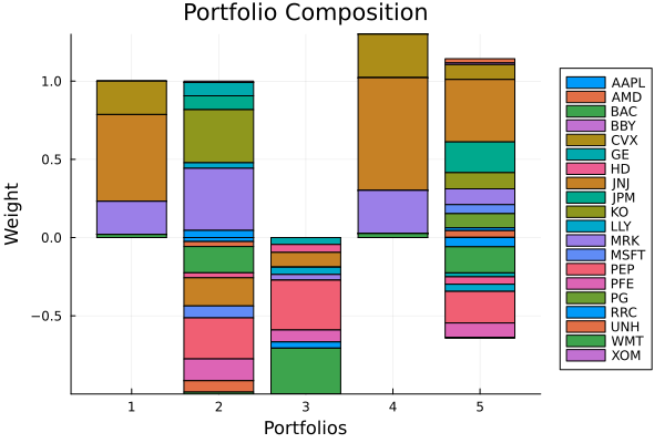
4. Budget ranges
A BudgetRange gives a lower and an upper bound on the budget or on the short budget. Each bound is 1.0 unless you give it. Pass nothing for a side that has no bound, but at least one of the two bounds must be a number. To put no constraint on the budget or the short budget, set bgt or sbgt to nothing.
We set a budget between 0.3 and 0.8 and a short budget of 0.5.
opt6 = JuMPOptimiser(; pe = pr, slv = slv, bgt = BudgetRange(; lb = 0.3, ub = 0.8), sbgt = 0.5, wb = WeightBounds(; lb = -1.0, ub = 1.0))mr6 = MeanRisk(; r = r, obj = MinimumRisk(), opt = opt6)res6 = optimise(mr6)println("budget: $(sum(res6.w))")println("long budget: $(sum(res6.w[res6.w .>= zero(eltype(res6.w))]))")println("short budget: $(sum(res6.w[res6.w .< zero(eltype(res6.w))]))")println("weight bounds: $(all(x -> -one(x) <= x <= one(x), res6.w))")budget: 0.30000000235617197
long budget: 0.6859015340047269
short budget: -0.38590153164855484
weight bounds: trueThe budget and the weight bounds are met, because they act on the weights. The short positions sum to less than 0.5 in size. The short budget acts on the relaxation variables, and each of them can sit above the short weight it covers.
Next we lower the short budget to 0.3.
opt7 = JuMPOptimiser(; pe = pr, slv = slv, bgt = BudgetRange(; lb = 0.3, ub = 0.8), sbgt = 0.3, wb = WeightBounds(; lb = -1.0, ub = 1.0))mr7 = MeanRisk(; r = r, obj = MinimumRisk(), opt = opt7)res7 = optimise(mr7)println("budget: $(sum(res7.w))")println("long budget: $(sum(res7.w[res7.w .>= zero(eltype(res7.w))]))")println("short budget: $(sum(res7.w[res7.w .< zero(eltype(res7.w))]))")println("weight bounds: $(all(x -> -one(x) <= x <= one(x), res7.w))")budget: 0.3000000056749746
long budget: 0.5999942896161827
short budget: -0.299994283941208
weight bounds: trueWe plot the weights of the two portfolios side by side.
plot_stacked_bar_composition([res6, res7], rd)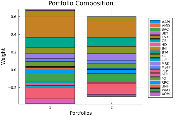
A short budget changes the weights only when it is smaller than the short exposure that the portfolio takes without it. The short positions of the first portfolio sum to more than 0.3 in size. Compare the short budget that the second cell prints with 0.3, and compare the two bars of the plot.
This page was generated using Literate.jl.