The source files can be found in user_guide/.
Constraints and costs
Real mandates are not unconstrained. You cap concentration, hold a sector band, limit how much you trade at each rebalance, and pay transaction costs. In PortfolioOptimisers.jl these are keywords on the JuMPOptimiser — the optimiser carries the constraints and costs, the estimator carries the objective. This page shows the common ones with one minimal call each; for the full treatment see the constraints & costs examples.
We fix one empirical prior and a minimum-risk objective so each keyword's effect is visible against the same baseline.
using PortfolioOptimisers, CSV, TimeSeries, DataFrames, PrettyTables, Clarabel, StatsPlots, GraphRecipesresfmt = (v, i, j) -> begin return if j == 1 v else isa(v, AbstractFloat) ? "$(round(v*100, digits=3)) %" : v endend;X = TimeArray(CSV.File(joinpath(@__DIR__, "../examples/SP500.csv.gz")); timestamp = :Date)[(end - 252):end]rd = prices_to_returns(X)pr = prior(EmpiricalPrior(), rd)slv = Solver(; name = :clarabel, solver = Clarabel.Optimizer, settings = Dict("verbose" => false), check_sol = (; allow_local = true, allow_almost = true))res_base = optimise(MeanRisk(; obj = MinimumRisk(), opt = JuMPOptimiser(; pe = pr, slv = slv)))MeanRiskResult
jr ┼ JuMPOptimisationResult
│ pa ┼ ProcessedJuMPOptimiserAttributes
│ │ pr ┼ LowOrderPrior
│ │ │ X ┼ 252×20 Matrix{Float64}
│ │ │ o_X ┼ nothing
│ │ │ mu ┼ 20-element Vector{Float64}
│ │ │ sigma ┼ 20×20 Matrix{Float64}
│ │ │ chol ┼ nothing
│ │ │ w ┼ nothing
│ │ │ ens ┼ nothing
│ │ │ kld ┼ nothing
│ │ │ ow ┼ nothing
│ │ │ rr ┼ nothing
│ │ │ fpr ┴ nothing
│ │ wb ┼ WeightBounds
│ │ │ lb ┼ 20-element StepRangeLen{Float64, Base.TwicePrecision{Float64}, Base.TwicePrecision{Float64}, Int64}
│ │ │ ub ┴ 20-element StepRangeLen{Float64, Base.TwicePrecision{Float64}, Base.TwicePrecision{Float64}, Int64}
│ │ lt ┼ nothing
│ │ st ┼ nothing
│ │ lcsr ┼ nothing
│ │ ctr ┼ nothing
│ │ gcardr ┼ nothing
│ │ sgcardr ┼ nothing
│ │ smtx ┼ nothing
│ │ sgmtx ┼ nothing
│ │ slt ┼ nothing
│ │ sst ┼ nothing
│ │ sglt ┼ nothing
│ │ sgst ┼ nothing
│ │ tn ┼ nothing
│ │ fees ┼ nothing
│ │ plr ┼ nothing
│ │ ret ┼ ArithmeticReturn
│ │ │ settings ┼ JuMPReturnsSettings
│ │ │ │ scale ┼ Float64: 1.0
│ │ │ │ lb ┼ nothing
│ │ │ │ rte ┼ Bool: true
│ │ │ │ fee ┼ Bool: true
│ │ │ │ mic ┴ Bool: true
│ │ │ ucs ┼ nothing
│ │ │ mu ┴ 20-element Vector{Float64}
│ │ sca ┼ SumScalariser()
│ │ imsk ┴ nothing
│ retcode ┼ OptimisationSuccess
│ │ res ┴ Dict{Any, Any}: Dict{Any, Any}()
│ sol ┼ JuMPOptimisationSolution
│ │ w ┴ 20-element Vector{Float64}
│ model ┼ A JuMP Model
│ │ ├ solver: Clarabel
│ │ ├ objective_sense: MIN_SENSE
│ │ │ └ objective_function_type: QuadExpr
│ │ ├ num_variables: 21
│ │ ├ num_constraints: 4
│ │ │ ├ AffExpr in MOI.EqualTo{Float64}: 1
│ │ │ ├ Vector{AffExpr} in MOI.Nonnegatives: 1
│ │ │ ├ Vector{AffExpr} in MOI.Nonpositives: 1
│ │ │ └ Vector{AffExpr} in MOI.SecondOrderCone: 1
│ │ └ Names registered in the model
│ │ └ :G, :T, :bgt, :cdev_soc_1, :dev_1, :k, :lw, :obj_expr, :ret, :ret_1, :ret_vec, :risk, :risk_vec, :sc, :so, :variance_flag, :variance_risk_1, :w, :w_lb, :w_ub
r ┼ Variance
│ settings ┼ RiskMeasureSettings
│ │ scale ┼ Float64: 1.0
│ │ ub ┼ nothing
│ │ rke ┴ Bool: true
│ sigma ┼ 20×20 Matrix{Float64}
│ chol ┼ nothing
│ rc ┼ nothing
│ alg ┴ SquaredSOCRiskExpr()
fb ┴ nothing
1. Weight bounds
WeightBounds sets the per-asset lower and upper bound through the wb keyword. The default is lb = 0, ub = 1 (long-only, fully invested). Capping ub forces diversification — no single name can exceed the bound.
res_cap = optimise(MeanRisk(; obj = MinimumRisk(), opt = JuMPOptimiser(; pe = pr, slv = slv, wb = WeightBounds(; lb = 0.0, ub = 0.10))))MeanRiskResult
jr ┼ JuMPOptimisationResult
│ pa ┼ ProcessedJuMPOptimiserAttributes
│ │ pr ┼ LowOrderPrior
│ │ │ X ┼ 252×20 Matrix{Float64}
│ │ │ o_X ┼ nothing
│ │ │ mu ┼ 20-element Vector{Float64}
│ │ │ sigma ┼ 20×20 Matrix{Float64}
│ │ │ chol ┼ nothing
│ │ │ w ┼ nothing
│ │ │ ens ┼ nothing
│ │ │ kld ┼ nothing
│ │ │ ow ┼ nothing
│ │ │ rr ┼ nothing
│ │ │ fpr ┴ nothing
│ │ wb ┼ WeightBounds
│ │ │ lb ┼ 20-element StepRangeLen{Float64, Base.TwicePrecision{Float64}, Base.TwicePrecision{Float64}, Int64}
│ │ │ ub ┴ 20-element StepRangeLen{Float64, Base.TwicePrecision{Float64}, Base.TwicePrecision{Float64}, Int64}
│ │ lt ┼ nothing
│ │ st ┼ nothing
│ │ lcsr ┼ nothing
│ │ ctr ┼ nothing
│ │ gcardr ┼ nothing
│ │ sgcardr ┼ nothing
│ │ smtx ┼ nothing
│ │ sgmtx ┼ nothing
│ │ slt ┼ nothing
│ │ sst ┼ nothing
│ │ sglt ┼ nothing
│ │ sgst ┼ nothing
│ │ tn ┼ nothing
│ │ fees ┼ nothing
│ │ plr ┼ nothing
│ │ ret ┼ ArithmeticReturn
│ │ │ settings ┼ JuMPReturnsSettings
│ │ │ │ scale ┼ Float64: 1.0
│ │ │ │ lb ┼ nothing
│ │ │ │ rte ┼ Bool: true
│ │ │ │ fee ┼ Bool: true
│ │ │ │ mic ┴ Bool: true
│ │ │ ucs ┼ nothing
│ │ │ mu ┴ 20-element Vector{Float64}
│ │ sca ┼ SumScalariser()
│ │ imsk ┴ nothing
│ retcode ┼ OptimisationSuccess
│ │ res ┴ Dict{Any, Any}: Dict{Any, Any}()
│ sol ┼ JuMPOptimisationSolution
│ │ w ┴ 20-element Vector{Float64}
│ model ┼ A JuMP Model
│ │ ├ solver: Clarabel
│ │ ├ objective_sense: MIN_SENSE
│ │ │ └ objective_function_type: QuadExpr
│ │ ├ num_variables: 21
│ │ ├ num_constraints: 4
│ │ │ ├ AffExpr in MOI.EqualTo{Float64}: 1
│ │ │ ├ Vector{AffExpr} in MOI.Nonnegatives: 1
│ │ │ ├ Vector{AffExpr} in MOI.Nonpositives: 1
│ │ │ └ Vector{AffExpr} in MOI.SecondOrderCone: 1
│ │ └ Names registered in the model
│ │ └ :G, :T, :bgt, :cdev_soc_1, :dev_1, :k, :lw, :obj_expr, :ret, :ret_1, :ret_vec, :risk, :risk_vec, :sc, :so, :variance_flag, :variance_risk_1, :w, :w_lb, :w_ub
r ┼ Variance
│ settings ┼ RiskMeasureSettings
│ │ scale ┼ Float64: 1.0
│ │ ub ┼ nothing
│ │ rke ┴ Bool: true
│ sigma ┼ 20×20 Matrix{Float64}
│ chol ┼ nothing
│ rc ┼ nothing
│ alg ┴ SquaredSOCRiskExpr()
fb ┴ nothing
The budget itself is the bgt keyword (default 1.0); BudgetRange and a separate short budget sbgt let you build long/short and leveraged mandates — see Budget Constraints.
2. Linear and group constraints
Group and linear constraints are written as plain strings over a UniverseSets and passed through lcse as a LinearConstraintEstimator — the same syntax used for views. Name a group, then bound it. Here we require the tech group to hold at least 15% (a floor the unconstrained minimum-risk portfolio would not give it).
sets = UniverseSets(; dict = Dict("nx" => rd.nx, "tech" => ["AAPL", "AMD", "MSFT"]))res_grp = optimise(MeanRisk(; obj = MinimumRisk(), opt = JuMPOptimiser(; pe = pr, slv = slv, sets = sets, lcse = LinearConstraintEstimator(; val = ["tech >= 0.15"]))))MeanRiskResult
jr ┼ JuMPOptimisationResult
│ pa ┼ ProcessedJuMPOptimiserAttributes
│ │ pr ┼ LowOrderPrior
│ │ │ X ┼ 252×20 Matrix{Float64}
│ │ │ o_X ┼ nothing
│ │ │ mu ┼ 20-element Vector{Float64}
│ │ │ sigma ┼ 20×20 Matrix{Float64}
│ │ │ chol ┼ nothing
│ │ │ w ┼ nothing
│ │ │ ens ┼ nothing
│ │ │ kld ┼ nothing
│ │ │ ow ┼ nothing
│ │ │ rr ┼ nothing
│ │ │ fpr ┴ nothing
│ │ wb ┼ WeightBounds
│ │ │ lb ┼ 20-element StepRangeLen{Float64, Base.TwicePrecision{Float64}, Base.TwicePrecision{Float64}, Int64}
│ │ │ ub ┴ 20-element StepRangeLen{Float64, Base.TwicePrecision{Float64}, Base.TwicePrecision{Float64}, Int64}
│ │ lt ┼ nothing
│ │ st ┼ nothing
│ │ lcsr ┼ LinearConstraint
│ │ │ ineq ┼ PartialLinearConstraint
│ │ │ │ A ┼ 1×20 LinearAlgebra.Transpose{Float64, Matrix{Float64}}
│ │ │ │ B ┴ Vector{Float64}: [-0.15]
│ │ │ eq ┴ nothing
│ │ ctr ┼ nothing
│ │ gcardr ┼ nothing
│ │ sgcardr ┼ nothing
│ │ smtx ┼ nothing
│ │ sgmtx ┼ nothing
│ │ slt ┼ nothing
│ │ sst ┼ nothing
│ │ sglt ┼ nothing
│ │ sgst ┼ nothing
│ │ tn ┼ nothing
│ │ fees ┼ nothing
│ │ plr ┼ nothing
│ │ ret ┼ ArithmeticReturn
│ │ │ settings ┼ JuMPReturnsSettings
│ │ │ │ scale ┼ Float64: 1.0
│ │ │ │ lb ┼ nothing
│ │ │ │ rte ┼ Bool: true
│ │ │ │ fee ┼ Bool: true
│ │ │ │ mic ┴ Bool: true
│ │ │ ucs ┼ nothing
│ │ │ mu ┴ 20-element Vector{Float64}
│ │ sca ┼ SumScalariser()
│ │ imsk ┴ nothing
│ retcode ┼ OptimisationSuccess
│ │ res ┴ Dict{Any, Any}: Dict{Any, Any}()
│ sol ┼ JuMPOptimisationSolution
│ │ w ┴ 20-element Vector{Float64}
│ model ┼ A JuMP Model
│ │ ├ solver: Clarabel
│ │ ├ objective_sense: MIN_SENSE
│ │ │ └ objective_function_type: QuadExpr
│ │ ├ num_variables: 21
│ │ ├ num_constraints: 5
│ │ │ ├ AffExpr in MOI.EqualTo{Float64}: 1
│ │ │ ├ Vector{AffExpr} in MOI.Nonnegatives: 1
│ │ │ ├ Vector{AffExpr} in MOI.Nonpositives: 2
│ │ │ └ Vector{AffExpr} in MOI.SecondOrderCone: 1
│ │ └ Names registered in the model
│ │ └ :G, :T, :bgt, :cdev_soc_1, :dev_1, :k, :lcs_ineq_1, :lw, :obj_expr, :ret, :ret_1, :ret_vec, :risk, :risk_vec, :sc, :so, :variance_flag, :variance_risk_1, :w, :w_lb, :w_ub
r ┼ Variance
│ settings ┼ RiskMeasureSettings
│ │ scale ┼ Float64: 1.0
│ │ ub ┼ nothing
│ │ rke ┴ Bool: true
│ sigma ┼ 20×20 Matrix{Float64}
│ chol ┼ nothing
│ rc ┼ nothing
│ alg ┴ SquaredSOCRiskExpr()
fb ┴ nothing
The same lcse handles absolute and relative bounds ("AAPL <= 0.1", "MSFT >= AMD"). For constraints built from the asset hierarchy — phylogeny and centrality — see Phylogeny & Centrality.
3. Factor exposure constraints
Real mandates are often written in factor names rather than tickers — "at most 10% momentum", "market-neutral to value". Those bound the portfolio's factor weights w_f = Mᵀw, where M is the loadings matrix a factor model already computes.
Wrap a LinearConstraintEstimator in an ExposureConstraintEstimator and declare the space with FactorSpace; the names resolve against the factor axis the loadings name, which for a time-series regression is the one a UniverseSets declares under tfkey (default "nf"), and the rows are projected through the loadings while the constraint is generated. What the optimiser receives is an ordinary asset-space constraint, so this composes with everything else on this page.
It needs loadings from somewhere, and factor data, which prices_to_returns takes as an optional second argument. By default the loadings come from the prior, so this wants FactorPrior rather than EmpiricalPrior — and a prior with no regression is an error, never a silently dropped row. The space can also supply its own: FactorSpace(; re = StepwiseRegression()) fits the loadings itself, which makes the mandate legal on any prior, and FactorSpace(; re = <a fitted Regression>) pins them. The deep dive covers the precedence and when a pinned basis goes stale.
Fac = TimeArray(CSV.File(joinpath(@__DIR__, "../examples/Factors.csv.gz")); timestamp = :Date)[(end - 252):end]rd_f = prices_to_returns(price_ingestion(PriceIngestion(), X; F = Fac))sets_f = UniverseSets(; dict = Dict("nx" => rd_f.nx, "nf" => rd_f.nf))res_fac = optimise(MeanRisk(; obj = MinimumRisk(), opt = JuMPOptimiser(; pe = FactorPrior(), slv = slv, sets = sets_f, lcse = ExposureConstraintEstimator(; lce = LinearConstraintEstimator(; val = "MTUM >= 0.2"), space = FactorSpace()))), rd_f)MeanRiskResult
jr ┼ JuMPOptimisationResult
│ pa ┼ ProcessedJuMPOptimiserAttributes
│ │ pr ┼ LowOrderPrior
│ │ │ X ┼ 252×20 Matrix{Float64}
│ │ │ o_X ┼ 252×20 Matrix{Float64}
│ │ │ mu ┼ 20-element Vector{Float64}
│ │ │ sigma ┼ 20×20 Matrix{Float64}
│ │ │ chol ┼ 25×20 LinearAlgebra.Transpose{Float64, Matrix{Float64}}
│ │ │ w ┼ nothing
│ │ │ ens ┼ nothing
│ │ │ kld ┼ nothing
│ │ │ ow ┼ nothing
│ │ │ rr ┼ Regression
│ │ │ │ M ┼ 20×5 SubArray{Float64, 2, Matrix{Float64}, Tuple{Base.Slice{Base.OneTo{Int64}}, UnitRange{Int64}}, true}
│ │ │ │ L ┼ 20×5 SubArray{Float64, 2, Matrix{Float64}, Tuple{Base.Slice{Base.OneTo{Int64}}, UnitRange{Int64}}, true}
│ │ │ │ b ┼ 20-element SubArray{Float64, 1, Matrix{Float64}, Tuple{Base.Slice{Base.OneTo{Int64}}, Int64}, true}
│ │ │ │ esigma ┴ 20-element Vector{Float64}
│ │ │ fpr ┼ LowOrderPrior
│ │ │ │ X ┼ 252×5 Matrix{Float64}
│ │ │ │ o_X ┼ nothing
│ │ │ │ mu ┼ Vector{Float64}: [-0.0007221367902182357, -0.0008384535501032073, -0.0006253517821839465, -0.0003358529620217417, -0.000559091885073412]
│ │ │ │ sigma ┼ 5×5 Matrix{Float64}
│ │ │ │ chol ┼ nothing
│ │ │ │ w ┼ nothing
│ │ │ │ ens ┼ nothing
│ │ │ │ kld ┼ nothing
│ │ │ │ ow ┼ nothing
│ │ │ │ rr ┼ nothing
│ │ │ │ fpr ┴ nothing
│ │ wb ┼ WeightBounds
│ │ │ lb ┼ 20-element StepRangeLen{Float64, Base.TwicePrecision{Float64}, Base.TwicePrecision{Float64}, Int64}
│ │ │ ub ┴ 20-element StepRangeLen{Float64, Base.TwicePrecision{Float64}, Base.TwicePrecision{Float64}, Int64}
│ │ lt ┼ nothing
│ │ st ┼ nothing
│ │ lcsr ┼ LinearConstraint
│ │ │ ineq ┼ PartialLinearConstraint
│ │ │ │ A ┼ 1×20 LinearAlgebra.Transpose{Float64, Matrix{Float64}}
│ │ │ │ B ┴ Vector{Float64}: [-0.2]
│ │ │ eq ┴ nothing
│ │ ctr ┼ nothing
│ │ gcardr ┼ nothing
│ │ sgcardr ┼ nothing
│ │ smtx ┼ nothing
│ │ sgmtx ┼ nothing
│ │ slt ┼ nothing
│ │ sst ┼ nothing
│ │ sglt ┼ nothing
│ │ sgst ┼ nothing
│ │ tn ┼ nothing
│ │ fees ┼ nothing
│ │ plr ┼ nothing
│ │ ret ┼ ArithmeticReturn
│ │ │ settings ┼ JuMPReturnsSettings
│ │ │ │ scale ┼ Float64: 1.0
│ │ │ │ lb ┼ nothing
│ │ │ │ rte ┼ Bool: true
│ │ │ │ fee ┼ Bool: true
│ │ │ │ mic ┴ Bool: true
│ │ │ ucs ┼ nothing
│ │ │ mu ┴ 20-element Vector{Float64}
│ │ sca ┼ SumScalariser()
│ │ imsk ┴ nothing
│ retcode ┼ OptimisationSuccess
│ │ res ┴ Dict{Any, Any}: Dict{Any, Any}()
│ sol ┼ JuMPOptimisationSolution
│ │ w ┴ 20-element Vector{Float64}
│ model ┼ A JuMP Model
│ │ ├ solver: Clarabel
│ │ ├ objective_sense: MIN_SENSE
│ │ │ └ objective_function_type: QuadExpr
│ │ ├ num_variables: 21
│ │ ├ num_constraints: 5
│ │ │ ├ AffExpr in MOI.EqualTo{Float64}: 1
│ │ │ ├ Vector{AffExpr} in MOI.Nonnegatives: 1
│ │ │ ├ Vector{AffExpr} in MOI.Nonpositives: 2
│ │ │ └ Vector{AffExpr} in MOI.SecondOrderCone: 1
│ │ └ Names registered in the model
│ │ └ :G, :T, :bgt, :cdev_soc_1, :dev_1, :k, :lcs_ineq_1, :lw, :obj_expr, :ret, :ret_1, :ret_vec, :risk, :risk_vec, :sc, :so, :variance_flag, :variance_risk_1, :w, :w_lb, :w_ub
r ┼ Variance
│ settings ┼ RiskMeasureSettings
│ │ scale ┼ Float64: 1.0
│ │ ub ┼ nothing
│ │ rke ┴ Bool: true
│ sigma ┼ 20×20 Matrix{Float64}
│ chol ┼ 25×20 LinearAlgebra.Transpose{Float64, Matrix{Float64}}
│ rc ┼ nothing
│ alg ┴ SquaredSOCRiskExpr()
fb ┴ nothing
Verify it by computing the realised exposures from the result — the loadings the optimiser actually used are on its prior:
pretty_table(DataFrame("Factor" => rd_f.nf, "Exposure" => transpose(res_fac.pa.pr.rr.M) * res_fac.w); formatters = [resfmt], title = "Realised factor exposures")Realised factor exposures
┌────────┬───────────┐
│ Factor │ Exposure │
│ String │ Float64 │
├────────┼───────────┤
│ MTUM │ 20.0 % │
│ QUAL │ -35.285 % │
│ SIZE │ -48.777 % │
│ USMV │ 96.28 % │
│ VLUE │ 49.392 % │
└────────┴───────────┘Pass the prior estimator, not a precomputed prior: the projection is then recomputed inside every cross-validation fold, against the loadings that fold actually fitted. This is the one constraint that cannot be precomputed by hand without going stale, and Factor Exposure Constraints measures how far a hand-written row drifts. It also covers factor groups, mixing factor- and asset-space rows, and which constraints have no factor form — the rule is that a constraint is re-based only if it is a linear row in w, so cardinality, thresholds, weight bounds, turnover, tracking error and fees all stay out, each for its own reason. Tracking a factor is the case that looks like a gap and is not: ReturnsTracking takes a benchmark return series, and a factor's return series is a column of the factor matrix, so it needs no re-basis at all.
4. Turnover
Costs enter the same way. Turnover (tn) limits how far the new weights may drift from a reference portfolio w — your current holdings — so a rebalance stays cheap. Here we anchor at the current minimum-risk portfolio and re-solve under a turnover budget.
res_tn = optimise(MeanRisk(; obj = MinimumRisk(), opt = JuMPOptimiser(; pe = pr, slv = slv, tn = Turnover(; w = res_base.w, val = 0.02))))MeanRiskResult
jr ┼ JuMPOptimisationResult
│ pa ┼ ProcessedJuMPOptimiserAttributes
│ │ pr ┼ LowOrderPrior
│ │ │ X ┼ 252×20 Matrix{Float64}
│ │ │ o_X ┼ nothing
│ │ │ mu ┼ 20-element Vector{Float64}
│ │ │ sigma ┼ 20×20 Matrix{Float64}
│ │ │ chol ┼ nothing
│ │ │ w ┼ nothing
│ │ │ ens ┼ nothing
│ │ │ kld ┼ nothing
│ │ │ ow ┼ nothing
│ │ │ rr ┼ nothing
│ │ │ fpr ┴ nothing
│ │ wb ┼ WeightBounds
│ │ │ lb ┼ 20-element StepRangeLen{Float64, Base.TwicePrecision{Float64}, Base.TwicePrecision{Float64}, Int64}
│ │ │ ub ┴ 20-element StepRangeLen{Float64, Base.TwicePrecision{Float64}, Base.TwicePrecision{Float64}, Int64}
│ │ lt ┼ nothing
│ │ st ┼ nothing
│ │ lcsr ┼ nothing
│ │ ctr ┼ nothing
│ │ gcardr ┼ nothing
│ │ sgcardr ┼ nothing
│ │ smtx ┼ nothing
│ │ sgmtx ┼ nothing
│ │ slt ┼ nothing
│ │ sst ┼ nothing
│ │ sglt ┼ nothing
│ │ sgst ┼ nothing
│ │ tn ┼ Turnover
│ │ │ w ┼ 20-element Vector{Float64}
│ │ │ val ┼ Float64: 0.02
│ │ │ fixed ┴ Bool: false
│ │ fees ┼ nothing
│ │ plr ┼ nothing
│ │ ret ┼ ArithmeticReturn
│ │ │ settings ┼ JuMPReturnsSettings
│ │ │ │ scale ┼ Float64: 1.0
│ │ │ │ lb ┼ nothing
│ │ │ │ rte ┼ Bool: true
│ │ │ │ fee ┼ Bool: true
│ │ │ │ mic ┴ Bool: true
│ │ │ ucs ┼ nothing
│ │ │ mu ┴ 20-element Vector{Float64}
│ │ sca ┼ SumScalariser()
│ │ imsk ┴ nothing
│ retcode ┼ OptimisationSuccess
│ │ res ┴ Dict{Any, Any}: Dict{Any, Any}()
│ sol ┼ JuMPOptimisationSolution
│ │ w ┴ 20-element Vector{Float64}
│ model ┼ A JuMP Model
│ │ ├ solver: Clarabel
│ │ ├ objective_sense: MIN_SENSE
│ │ │ └ objective_function_type: QuadExpr
│ │ ├ num_variables: 41
│ │ ├ num_constraints: 25
│ │ │ ├ AffExpr in MOI.EqualTo{Float64}: 1
│ │ │ ├ Vector{AffExpr} in MOI.Nonnegatives: 1
│ │ │ ├ Vector{AffExpr} in MOI.Nonpositives: 2
│ │ │ ├ Vector{AffExpr} in MOI.NormOneCone: 20
│ │ │ └ Vector{AffExpr} in MOI.SecondOrderCone: 1
│ │ └ Names registered in the model
│ │ └ :G, :T, :bgt, :cdev_soc_1, :ctn_1, :ctn_noc_1, :dev_1, :k, :lw, :obj_expr, :ret, :ret_1, :ret_vec, :risk, :risk_vec, :sc, :so, :t_tn_1, :tn_1, :variance_flag, :variance_risk_1, :w, :w_lb, :w_ub
r ┼ Variance
│ settings ┼ RiskMeasureSettings
│ │ scale ┼ Float64: 1.0
│ │ ub ┼ nothing
│ │ rke ┴ Bool: true
│ sigma ┼ 20×20 Matrix{Float64}
│ chol ┼ nothing
│ rc ┼ nothing
│ alg ┴ SquaredSOCRiskExpr()
fb ┴ nothing
A tighter val keeps the result closer to the reference holdings; a looser one frees the optimiser to move toward the unconstrained solution.
5. Fees
Fees (fees) charges proportional (and optionally fixed) transaction costs on long and short positions, which the objective then trades off against return. The minimal form sets a per-unit long fee.
res_fee = optimise(MeanRisk(; obj = MaximumRatio(; rf = 4.2 / 100 / 252), opt = JuMPOptimiser(; pe = pr, slv = slv, fees = Fees(; l = 0.001))))MeanRiskResult
jr ┼ JuMPOptimisationResult
│ pa ┼ ProcessedJuMPOptimiserAttributes
│ │ pr ┼ LowOrderPrior
│ │ │ X ┼ 252×20 Matrix{Float64}
│ │ │ o_X ┼ nothing
│ │ │ mu ┼ 20-element Vector{Float64}
│ │ │ sigma ┼ 20×20 Matrix{Float64}
│ │ │ chol ┼ nothing
│ │ │ w ┼ nothing
│ │ │ ens ┼ nothing
│ │ │ kld ┼ nothing
│ │ │ ow ┼ nothing
│ │ │ rr ┼ nothing
│ │ │ fpr ┴ nothing
│ │ wb ┼ WeightBounds
│ │ │ lb ┼ 20-element StepRangeLen{Float64, Base.TwicePrecision{Float64}, Base.TwicePrecision{Float64}, Int64}
│ │ │ ub ┴ 20-element StepRangeLen{Float64, Base.TwicePrecision{Float64}, Base.TwicePrecision{Float64}, Int64}
│ │ lt ┼ nothing
│ │ st ┼ nothing
│ │ lcsr ┼ nothing
│ │ ctr ┼ nothing
│ │ gcardr ┼ nothing
│ │ sgcardr ┼ nothing
│ │ smtx ┼ nothing
│ │ sgmtx ┼ nothing
│ │ slt ┼ nothing
│ │ sst ┼ nothing
│ │ sglt ┼ nothing
│ │ sgst ┼ nothing
│ │ tn ┼ nothing
│ │ fees ┼ Fees
│ │ │ tn ┼ nothing
│ │ │ l ┼ Float64: 0.001
│ │ │ s ┼ nothing
│ │ │ fl ┼ nothing
│ │ │ fs ┼ nothing
│ │ │ lq ┼ nothing
│ │ │ flq ┼ nothing
│ │ │ fa ┼ nothing
│ │ │ kwargs ┴ @NamedTuple{atol::Float64}: (atol = 1.0e-8,)
│ │ plr ┼ nothing
│ │ ret ┼ ArithmeticReturn
│ │ │ settings ┼ JuMPReturnsSettings
│ │ │ │ scale ┼ Float64: 1.0
│ │ │ │ lb ┼ nothing
│ │ │ │ rte ┼ Bool: true
│ │ │ │ fee ┼ Bool: true
│ │ │ │ mic ┴ Bool: true
│ │ │ ucs ┼ nothing
│ │ │ mu ┴ 20-element Vector{Float64}
│ │ sca ┼ SumScalariser()
│ │ imsk ┴ nothing
│ retcode ┼ OptimisationSuccess
│ │ res ┴ Dict{Any, Any}: Dict{Any, Any}()
│ sol ┼ JuMPOptimisationSolution
│ │ w ┴ 20-element Vector{Float64}
│ model ┼ A JuMP Model
│ │ ├ solver: Clarabel
│ │ ├ objective_sense: MIN_SENSE
│ │ │ └ objective_function_type: QuadExpr
│ │ ├ num_variables: 22
│ │ ├ num_constraints: 6
│ │ │ ├ AffExpr in MOI.EqualTo{Float64}: 2
│ │ │ ├ Vector{AffExpr} in MOI.Nonnegatives: 1
│ │ │ ├ Vector{AffExpr} in MOI.Nonpositives: 1
│ │ │ ├ Vector{AffExpr} in MOI.SecondOrderCone: 1
│ │ │ └ VariableRef in MOI.GreaterThan{Float64}: 1
│ │ └ Names registered in the model
│ │ └ :G, :T, :bgt, :cdev_soc_1, :dev_1, :fee_fa, :fees, :fl, :k, :lw, :obj_expr, :ohf, :ret, :ret_1, :ret_vec, :risk, :risk_vec, :sc, :so, :sr_ret, :variance_flag, :variance_risk_1, :w, :w_lb, :w_ub
r ┼ Variance
│ settings ┼ RiskMeasureSettings
│ │ scale ┼ Float64: 1.0
│ │ ub ┼ nothing
│ │ rke ┴ Bool: true
│ sigma ┼ 20×20 Matrix{Float64}
│ chol ┼ nothing
│ rc ┼ nothing
│ alg ┴ SquaredSOCRiskExpr()
fb ┴ nothing
Soft alternatives to hard turnover/position limits — L1/L2 weight regularisation and a weight-norm ceiling that doubles as a diversification floor (l1, l2, l2c) — are covered in Regularisation; benchmark TrackingError (the tr keyword) in Turnover & Tracking.
6. Custom objectives and constraints
When a mandate needs something no built-in keyword covers — a continuous per-asset preference like a factor score, or a relationship between weights that isn't a plain linear bound — two JuMPOptimiser extension points let you write straight against the JuMP model:
cobjtakes aCustomJuMPObjective— implementadd_custom_objective_term!to price a preference, contributing the term withadd_to_objective_penalty!.ccnttakes aCustomJuMPConstraint— implementadd_custom_constraint!to add a constraint to the model.
Each keyword takes a single estimator or a vector of them, and each hook dispatches on the estimator's type. The two hooks take the same arguments — (model, <what you dispatch on>, optimiser, attrs), with the objective one adding the ObjectiveFunction ahead of the dispatch argument. Subtyping one of these without implementing its method is an error, not a no-op, so a mis-shaped signature is caught rather than silently ignored.
Because a custom objective term goes through the objective penalty, the library applies the sign matching whichever optimisation sense is being built: a contribution always worsens the objective, and a reward is a negative contribution. One definition is therefore correct under every objective, MaximumRatio included. The custom objectives & constraints example builds both from scratch — a momentum tilt and a momentum floor — and works through the two model idioms (the constraint scale, and the homogenisation variable k) that keep a hand-written term correct.
7. Comparing the effect
Same prior, same objective — only the constraint or cost changes the allocation.
results = [res_base, res_cap, res_grp, res_tn, res_fee]labels = ["Base", "Cap 10%", "Tech ≥ 15%", "Turnover", "Fees"]pretty_table(DataFrame(["Asset" => rd.nx, [labels[i] => results[i].w for i in eachindex(results)]...]); formatters = [resfmt], title = "Weights under each constraint / cost")plot_stacked_bar_composition(results, rd; xticks = (1:length(labels), labels))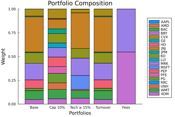
This page was generated using Literate.jl.