The source files can be found in examples/.
Maximum diversification
The diversification ratio of a portfolio is the weighted average of the volatilities of its assets, divided by the volatility of the portfolio.
\[\mathrm{DR}(\boldsymbol{w}) = \frac{\boldsymbol{w}^\intercal \boldsymbol{\sigma}}{\sqrt{\boldsymbol{w}^\intercal \mathbf{\Sigma} \boldsymbol{w}}}\,,\]
where $\boldsymbol{\sigma}$ is the vector of the volatilities of the assets and $\mathbf{\Sigma}$ is their covariance matrix. The ratio is one for a portfolio of one asset, and it grows as the correlations between the assets cut the risk of the portfolio. The maximum diversification portfolio maximises it.
The library has no optimiser of that name, and it needs none. The ratio is a MaximumRatio problem of MeanRisk:
- the numerator is the expected return of the portfolio, when the expected return of each asset is its volatility.
StandardDeviationExpectedReturnsgives this vector to the prior; - the denominator is the
StandardDeviationrisk measure; - the risk-free rate is zero, the default of
MaximumRatio.
This page builds the portfolio, checks that it has the largest diversification ratio, and compares it with the InverseVolatility and the minimum-variance portfolios.
Reach for the maximum diversification portfolio when you do not trust the estimates of the expected returns, but you want more than the minimum-variance portfolio. It uses only the covariance matrix, as the minimum-variance portfolio does, but it does not prefer the assets of low volatility. It prefers the assets of low correlation to the others.
using PortfolioOptimisers, CSV, TimeSeries, DataFrames, PrettyTables, Clarabel, HiGHS, Pajarito, JuMP, StatsPlots, LinearAlgebraresfmt = (v, i, j) -> begin if j == 1 return v else return isa(v, AbstractFloat) ? "$(round(v * 100, digits = 3)) %" : v endend;1. Data and the prior
We load the last 253 days of the S&P 500 prices that the other optimiser examples use, and compute their returns.
X = TimeArray(CSV.File(joinpath(@__DIR__, "..", "SP500.csv.gz")); timestamp = :Date)[(end - 252):end]rd = prices_to_returns(X)ReturnsResult
nx ┼ 20-element Vector{String}
X ┼ 252×20 Matrix{Float64}
nf ┼ nothing
F ┼ nothing
nb ┼ nothing
B ┼ nothing
ne ┼ nothing
E ┼ nothing
ts ┼ 252-element Vector{Date}
iv ┼ nothing
ivpa ┼ nothing
pnl ┴ nothing
The prior takes StandardDeviationExpectedReturns as its expected returns estimator, me. The mean vector of the prior is then the vector of the volatilities. Its covariance estimator has the same default as the covariance estimator of the prior, so $\boldsymbol{\sigma}$ is the square root of the diagonal of $\mathbf{\Sigma}$.
pr = prior(EmpiricalPrior(; me = StandardDeviationExpectedReturns()), rd)isapprox(pr.mu, sqrt.(diag(pr.sigma)))true2. The maximum diversification portfolio
The return measure of MeanRisk is ArithmeticReturn by default, and it reads the mean vector of the prior. So the expected return of the portfolio is $\boldsymbol{w}^\intercal \boldsymbol{\sigma}$, and MaximumRatio with rf = 0 maximises the diversification ratio.
The risk-free rate must be zero. A rate rf other than zero maximises $(\boldsymbol{w}^\intercal \boldsymbol{\sigma} - r_f) / \sqrt{\boldsymbol{w}^\intercal \mathbf{\Sigma} \boldsymbol{w}}$, which is a different problem with a different portfolio.
slv = Solver(; name = :clarabel1, solver = Clarabel.Optimizer, settings = Dict("verbose" => false), check_sol = (; allow_local = true, allow_almost = true))opt = JuMPOptimiser(; pe = pr, slv = slv)r = StandardDeviation()res_md = optimise(MeanRisk(; r = r, obj = MaximumRatio(), opt = opt))MeanRiskResult
jr ┼ JuMPOptimisationResult
│ jor ┼ ResolvedJuMPOptimiser
│ │ pr ┼ LowOrderPrior
│ │ │ X ┼ 252×20 Matrix{Float64}
│ │ │ o_X ┼ nothing
│ │ │ mu ┼ 20-element Vector{Float64}
│ │ │ sigma ┼ 20×20 Matrix{Float64}
│ │ │ chol ┼ nothing
│ │ │ w ┼ nothing
│ │ │ ens ┼ nothing
│ │ │ eoc ┼ Tuple{Nothing, Nothing}: (nothing, nothing)
│ │ │ kld ┼ nothing
│ │ │ ow ┼ nothing
│ │ │ rr ┼ nothing
│ │ │ fpr ┼ nothing
│ │ │ x_src ┼ nothing
│ │ │ ss_gaps ┼ nothing
│ │ │ pc ┴ nothing
│ │ fees ┼ nothing
│ │ ret ┼ ArithmeticReturn
│ │ │ settings ┼ JuMPReturnsSettings
│ │ │ │ scale ┼ Float64: 1.0
│ │ │ │ lb ┼ nothing
│ │ │ │ rte ┼ Bool: true
│ │ │ │ fee ┼ Bool: true
│ │ │ │ mic ┴ Bool: true
│ │ │ ucs ┼ nothing
│ │ │ mu ┼ 20-element Vector{Float64}
│ │ │ mtx_sqrt ┴ EigenFallbackSquareRoot()
│ │ sca ┼ nothing
│ │ imsk ┼ nothing
│ │ cbr ┼ ResolvedConstraintBlock
│ │ │ pr ┼ LowOrderPrior
│ │ │ │ X ┼ 252×20 Matrix{Float64}
│ │ │ │ o_X ┼ nothing
│ │ │ │ mu ┼ 20-element Vector{Float64}
│ │ │ │ sigma ┼ 20×20 Matrix{Float64}
│ │ │ │ chol ┼ nothing
│ │ │ │ w ┼ nothing
│ │ │ │ ens ┼ nothing
│ │ │ │ eoc ┼ Tuple{Nothing, Nothing}: (nothing, nothing)
│ │ │ │ kld ┼ nothing
│ │ │ │ ow ┼ nothing
│ │ │ │ rr ┼ nothing
│ │ │ │ fpr ┼ nothing
│ │ │ │ x_src ┼ nothing
│ │ │ │ ss_gaps ┼ nothing
│ │ │ │ pc ┴ nothing
│ │ │ rd ┼ ReturnsResult
│ │ │ │ nx ┼ nothing
│ │ │ │ X ┼ nothing
│ │ │ │ nf ┼ nothing
│ │ │ │ F ┼ nothing
│ │ │ │ nb ┼ nothing
│ │ │ │ B ┼ nothing
│ │ │ │ ne ┼ nothing
│ │ │ │ E ┼ nothing
│ │ │ │ ts ┼ nothing
│ │ │ │ iv ┼ nothing
│ │ │ │ ivpa ┼ nothing
│ │ │ │ pnl ┴ nothing
│ │ │ wb ┼ WeightBounds
│ │ │ │ lb ┼ 20-element StepRangeLen{Float64, Base.TwicePrecision{Float64}, Base.TwicePrecision{Float64}, Int64}
│ │ │ │ ub ┴ 20-element StepRangeLen{Float64, Base.TwicePrecision{Float64}, Base.TwicePrecision{Float64}, Int64}
│ │ │ lt ┼ nothing
│ │ │ st ┼ nothing
│ │ │ lcsr ┼ nothing
│ │ │ ctr ┼ nothing
│ │ │ gcardr ┼ nothing
│ │ │ sgcardr ┼ nothing
│ │ │ smtx ┼ nothing
│ │ │ sgmtx ┼ nothing
│ │ │ slt ┼ nothing
│ │ │ sst ┼ nothing
│ │ │ sglt ┼ nothing
│ │ │ sgst ┼ nothing
│ │ │ tn ┼ nothing
│ │ │ plr ┼ nothing
│ │ │ l2c ┼ nothing
│ │ │ lpc ┼ nothing
│ │ │ linfc ┼ nothing
│ │ │ l1 ┼ nothing
│ │ │ l2 ┼ nothing
│ │ │ lp ┼ nothing
│ │ │ linf ┼ nothing
│ │ │ card ┼ nothing
│ │ │ scard ┼ nothing
│ │ │ ss ┼ nothing
│ │ │ xbgt ┼ Bool: false
│ │ │ sbgt ┼ nothing
│ │ │ gbgt ┼ nothing
│ │ │ ccnt ┼ nothing
│ │ │ cobj ┴ nothing
│ retcode ┼ OptimisationSuccess
│ │ res ┴ Dict{Union{AbstractString, Symbol}, AbstractDict{Symbol}}: Dict{Union{AbstractString, Symbol}, AbstractDict{Symbol}}()
│ sol ┼ JuMPOptimisationSolution
│ │ w ┴ 20-element Vector{Float64}
│ model ┼ A JuMP Model
│ │ ├ solver: Clarabel
│ │ ├ objective_sense: MIN_SENSE
│ │ │ └ objective_function_type: AffExpr
│ │ ├ num_variables: 22
│ │ ├ num_constraints: 6
│ │ │ ├ AffExpr in MOI.EqualTo{Float64}: 2
│ │ │ ├ Vector{AffExpr} in MOI.Nonnegatives: 1
│ │ │ ├ Vector{AffExpr} in MOI.Nonpositives: 1
│ │ │ ├ Vector{AffExpr} in MOI.SecondOrderCone: 1
│ │ │ └ VariableRef in MOI.GreaterThan{Float64}: 1
│ │ └ Names registered in the model
│ │ └ :G, :T, :bgt, :csd_risk_soc_1, :k, :lw, :obj_expr, :ohf, :ret, :ret_1, :ret_vec, :risk, :risk_minimised, :risk_vec, :sc, :sd_risk_1, :sdp_corner, :so, :sr_ret, :w, :w_gross_ub, :w_lb, :w_ub
r ┼ StandardDeviation
│ settings ┼ RiskMeasureSettings
│ │ scale ┼ Float64: 1.0
│ │ ub ┼ nothing
│ │ rke ┴ Bool: true
│ sigma ┼ 20×20 Matrix{Float64}
│ chol ┼ nothing
│ mtx_sqrt ┴ EigenFallbackSquareRoot()
fb ┴ nothing
3. Three benchmarks
The minimum-variance portfolio uses the same risk measure and the same optimiser, with the MinimumRisk objective. The InverseVolatility portfolio gives each asset a weight in proportion to the inverse of its volatility. It needs no solver. The EqualWeighted portfolio gives each asset the same weight.
res_mv = optimise(MeanRisk(; r = r, obj = MinimumRisk(), opt = opt))res_iv = optimise(InverseVolatility(; pe = pr))res_ew = optimise(EqualWeighted(), rd)pretty_table(DataFrame(; :assets => rd.nx, Symbol("max diversification") => res_md.w, Symbol("min variance") => res_mv.w, Symbol("inverse volatility") => res_iv.w); formatters = [resfmt])┌────────┬─────────────────────┬──────────────┬────────────────────┐
│ assets │ max diversification │ min variance │ inverse volatility │
│ String │ Float64 │ Float64 │ Float64 │
├────────┼─────────────────────┼──────────────┼────────────────────┤
│ AAPL │ 0.0 % │ 0.0 % │ 4.004 % │
│ AMD │ 4.737 % │ 0.0 % │ 2.332 % │
│ BAC │ 1.092 % │ 0.0 % │ 4.39 % │
│ BBY │ 5.095 % │ 0.0 % │ 3.143 % │
│ CVX │ 0.918 % │ 7.415 % │ 4.326 % │
│ GE │ 3.53 % │ 0.822 % │ 4.087 % │
│ HD │ 0.0 % │ 0.0 % │ 4.55 % │
│ JNJ │ 7.082 % │ 36.972 % │ 8.175 % │
│ JPM │ 0.0 % │ 0.763 % │ 4.771 % │
│ KO │ 0.0 % │ 11.103 % │ 7.239 % │
│ LLY │ 4.901 % │ 0.0 % │ 5.224 % │
│ MRK │ 17.912 % │ 17.463 % │ 7.143 % │
│ MSFT │ 0.0 % │ 0.0 % │ 4.046 % │
│ PEP │ 0.0 % │ 8.973 % │ 7.32 % │
│ PFE │ 8.777 % │ 0.0 % │ 5.274 % │
│ PG │ 10.18 % │ 2.397 % │ 6.482 % │
│ RRC │ 7.431 % │ 0.0 % │ 2.263 % │
│ UNH │ 0.0 % │ 0.0 % │ 5.843 % │
│ WMT │ 17.843 % │ 9.356 % │ 5.329 % │
│ XOM │ 10.502 % │ 4.735 % │ 4.058 % │
└────────┴─────────────────────┴──────────────┴────────────────────┘4. The diversification ratio of each portfolio
expected_risk_ret_ratio returns the risk, the return and the ratio of a portfolio. With the prior of section 1, the return is $\boldsymbol{w}^\intercal \boldsymbol{\sigma}$, so the ratio is the diversification ratio. The default risk-free rate of the function is zero.
dr(w) = expected_risk_ret_ratio(r, ArithmeticReturn(), w, pr)[3]portfolios = ["max diversification" => res_md, "min variance" => res_mv, "inverse volatility" => res_iv, "equal weighted" => res_ew]pretty_table(DataFrame(; :portfolio => first.(portfolios), Symbol("diversification ratio") => [dr(p.w) for p in last.(portfolios)], :volatility => [expected_risk(r, p.w, pr) for p in last.(portfolios)], Symbol("assets held") => [count(>(1e-6), p.w) for p in last.(portfolios)]); formatters = [(v, i, j) -> j == 2 ? round(v; digits = 4) : resfmt(v, i, j)])┌─────────────────────┬───────────────────────┬────────────┬─────────────┐
│ portfolio │ diversification ratio │ volatility │ assets held │
│ String │ Float64 │ Float64 │ Int64 │
├─────────────────────┼───────────────────────┼────────────┼─────────────┤
│ max diversification │ 1.6974 │ 1.147 % │ 13 │
│ min variance │ 1.4467 │ 0.934 % │ 10 │
│ inverse volatility │ 1.5677 │ 1.143 % │ 20 │
│ equal weighted │ 1.5696 │ 1.283 % │ 20 │
└─────────────────────┴───────────────────────┴────────────┴─────────────┘The maximum diversification portfolio has the largest diversification ratio of the four.
all(dr(res_md.w) > dr(res.w) for res in (res_iv, res_mv, res_ew))trueThe minimum-variance portfolio has the lowest volatility, and the maximum diversification portfolio does not. The two portfolios answer different questions: the first asks for the least risk, and the second asks for the most risk that the correlations remove.
5. The minimum variance of the correlation matrix
Write the weights as $w_i = y_i / \sigma_i$, up to a positive scale. The diversification ratio is then $\sum_i y_i / \sqrt{\boldsymbol{y}^\intercal \mathbf{C} \boldsymbol{y}}$, where $\mathbf{C}$ is the correlation matrix. With the budget $\sum_i y_i = 1$, to maximise the ratio is to minimise the variance $\boldsymbol{y}^\intercal \mathbf{C} \boldsymbol{y}$. So the maximum diversification portfolio is the minimum-variance portfolio of the correlation matrix, divided by the volatilities and scaled to the budget.
CorrelationCovariance returns the correlation matrix of the estimator that it wraps, so a prior with it as ce has $\mathbf{C}$ in the place of $\mathbf{\Sigma}$. We solve the minimum-variance problem on that prior, and compare the result with the portfolio of section 2.
pr_cor = prior(EmpiricalPrior(; ce = CorrelationCovariance(; ce = PortfolioOptimisersCovariance())), rd)res_cor = optimise(MeanRisk(; r = r, obj = MinimumRisk(), opt = JuMPOptimiser(; pe = pr_cor, slv = slv)))w_cor = res_cor.w ./ pr.muw_cor ./= sum(w_cor)isapprox(w_cor, res_md.w; atol = 1e-4)trueThe two solves give the same weights, to the tolerance of the solver.
6. A cap on the number of assets
The maximum diversification portfolio of section 2 holds most of the assets. The card keyword of JuMPOptimiser caps the number of assets that hold a weight. It adds binary variables, so it needs a mixed-integer solver. We use Pajarito, which uses HiGHS for the integer part and Clarabel for the conic part, as the cardinality and threshold example does.
mip_slv = Solver(; name = :mip1, solver = optimizer_with_attributes(Pajarito.Optimizer, "verbose" => false, "oa_solver" => optimizer_with_attributes(HiGHS.Optimizer, JuMP.MOI.Silent() => true), "conic_solver" => optimizer_with_attributes(Clarabel.Optimizer, "verbose" => false)), check_sol = (; allow_local = true, allow_almost = true))k = 5res_card = optimise(MeanRisk(; r = r, obj = MaximumRatio(), opt = JuMPOptimiser(; pe = pr, slv = mip_slv, card = k)))MeanRiskResult
jr ┼ JuMPOptimisationResult
│ jor ┼ ResolvedJuMPOptimiser
│ │ pr ┼ LowOrderPrior
│ │ │ X ┼ 252×20 Matrix{Float64}
│ │ │ o_X ┼ nothing
│ │ │ mu ┼ 20-element Vector{Float64}
│ │ │ sigma ┼ 20×20 Matrix{Float64}
│ │ │ chol ┼ nothing
│ │ │ w ┼ nothing
│ │ │ ens ┼ nothing
│ │ │ eoc ┼ Tuple{Nothing, Nothing}: (nothing, nothing)
│ │ │ kld ┼ nothing
│ │ │ ow ┼ nothing
│ │ │ rr ┼ nothing
│ │ │ fpr ┼ nothing
│ │ │ x_src ┼ nothing
│ │ │ ss_gaps ┼ nothing
│ │ │ pc ┴ nothing
│ │ fees ┼ nothing
│ │ ret ┼ ArithmeticReturn
│ │ │ settings ┼ JuMPReturnsSettings
│ │ │ │ scale ┼ Float64: 1.0
│ │ │ │ lb ┼ nothing
│ │ │ │ rte ┼ Bool: true
│ │ │ │ fee ┼ Bool: true
│ │ │ │ mic ┴ Bool: true
│ │ │ ucs ┼ nothing
│ │ │ mu ┼ 20-element Vector{Float64}
│ │ │ mtx_sqrt ┴ EigenFallbackSquareRoot()
│ │ sca ┼ nothing
│ │ imsk ┼ nothing
│ │ cbr ┼ ResolvedConstraintBlock
│ │ │ pr ┼ LowOrderPrior
│ │ │ │ X ┼ 252×20 Matrix{Float64}
│ │ │ │ o_X ┼ nothing
│ │ │ │ mu ┼ 20-element Vector{Float64}
│ │ │ │ sigma ┼ 20×20 Matrix{Float64}
│ │ │ │ chol ┼ nothing
│ │ │ │ w ┼ nothing
│ │ │ │ ens ┼ nothing
│ │ │ │ eoc ┼ Tuple{Nothing, Nothing}: (nothing, nothing)
│ │ │ │ kld ┼ nothing
│ │ │ │ ow ┼ nothing
│ │ │ │ rr ┼ nothing
│ │ │ │ fpr ┼ nothing
│ │ │ │ x_src ┼ nothing
│ │ │ │ ss_gaps ┼ nothing
│ │ │ │ pc ┴ nothing
│ │ │ rd ┼ ReturnsResult
│ │ │ │ nx ┼ nothing
│ │ │ │ X ┼ nothing
│ │ │ │ nf ┼ nothing
│ │ │ │ F ┼ nothing
│ │ │ │ nb ┼ nothing
│ │ │ │ B ┼ nothing
│ │ │ │ ne ┼ nothing
│ │ │ │ E ┼ nothing
│ │ │ │ ts ┼ nothing
│ │ │ │ iv ┼ nothing
│ │ │ │ ivpa ┼ nothing
│ │ │ │ pnl ┴ nothing
│ │ │ wb ┼ WeightBounds
│ │ │ │ lb ┼ 20-element StepRangeLen{Float64, Base.TwicePrecision{Float64}, Base.TwicePrecision{Float64}, Int64}
│ │ │ │ ub ┴ 20-element StepRangeLen{Float64, Base.TwicePrecision{Float64}, Base.TwicePrecision{Float64}, Int64}
│ │ │ lt ┼ nothing
│ │ │ st ┼ nothing
│ │ │ lcsr ┼ nothing
│ │ │ ctr ┼ nothing
│ │ │ gcardr ┼ nothing
│ │ │ sgcardr ┼ nothing
│ │ │ smtx ┼ nothing
│ │ │ sgmtx ┼ nothing
│ │ │ slt ┼ nothing
│ │ │ sst ┼ nothing
│ │ │ sglt ┼ nothing
│ │ │ sgst ┼ nothing
│ │ │ tn ┼ nothing
│ │ │ plr ┼ nothing
│ │ │ l2c ┼ nothing
│ │ │ lpc ┼ nothing
│ │ │ linfc ┼ nothing
│ │ │ l1 ┼ nothing
│ │ │ l2 ┼ nothing
│ │ │ lp ┼ nothing
│ │ │ linf ┼ nothing
│ │ │ card ┼ Int64: 5
│ │ │ scard ┼ nothing
│ │ │ ss ┼ nothing
│ │ │ xbgt ┼ Bool: false
│ │ │ sbgt ┼ nothing
│ │ │ gbgt ┼ nothing
│ │ │ ccnt ┼ nothing
│ │ │ cobj ┴ nothing
│ retcode ┼ OptimisationSuccess
│ │ res ┴ Dict{Union{AbstractString, Symbol}, AbstractDict{Symbol}}: Dict{Union{AbstractString, Symbol}, AbstractDict{Symbol}}()
│ sol ┼ JuMPOptimisationSolution
│ │ w ┴ 20-element Vector{Float64}
│ model ┼ A JuMP Model
│ │ ├ solver: Pajarito
│ │ ├ objective_sense: MIN_SENSE
│ │ │ └ objective_function_type: AffExpr
│ │ ├ num_variables: 62
│ │ ├ num_constraints: 52
│ │ │ ├ AffExpr in MOI.EqualTo{Float64}: 2
│ │ │ ├ AffExpr in MOI.LessThan{Float64}: 1
│ │ │ ├ Vector{AffExpr} in MOI.Nonnegatives: 3
│ │ │ ├ Vector{AffExpr} in MOI.Nonpositives: 4
│ │ │ ├ Vector{AffExpr} in MOI.SecondOrderCone: 1
│ │ │ ├ VariableRef in MOI.GreaterThan{Float64}: 21
│ │ │ └ VariableRef in MOI.ZeroOne: 20
│ │ └ Names registered in the model
│ │ └ :G, :T, :bgt, :card, :csd_risk_soc_1, :i_mip, :ib, :ibf, :ibf_ub, :ibfd_lb, :ibfd_ub, :k, :lw, :mip_indicators, :obj_expr, :ohf, :ret, :ret_1, :ret_vec, :risk, :risk_minimised, :risk_vec, :sc, :sd_risk_1, :sdp_corner, :so, :sr_ret, :ss, :w, :w_gross_ub, :w_lb, :w_mip_lb, :w_mip_ub, :w_ub
r ┼ StandardDeviation
│ settings ┼ RiskMeasureSettings
│ │ scale ┼ Float64: 1.0
│ │ ub ┼ nothing
│ │ rke ┴ Bool: true
│ sigma ┼ 20×20 Matrix{Float64}
│ chol ┼ nothing
│ mtx_sqrt ┴ EigenFallbackSquareRoot()
fb ┴ nothing
An L1UncertaintySet gives a portfolio of k assets with no binary variables. The ℓ1 uncertainty sets example shows the model. MaximumReturn with NoRisk maximises the worst-case return over the set, and the result holds the k assets with the highest characteristic, with equal weights. It is a linear program, so HiGHS solves it alone.
The set must be centred on the return term of this page, the volatilities. So its prior takes StandardDeviationExpectedReturns, as the prior of section 1 does. ActiveAssetsUncertaintyAlgorithm finds the radius that makes k assets active.
ue = CharacteristicUncertaintySet(; pe = EmpiricalPrior(; me = StandardDeviationExpectedReturns()), alg = L1UncertaintySetAlgorithm(; method = ActiveAssetsUncertaintyAlgorithm(; active = CountOf(k))))lp_slv = Solver(; name = :highs, solver = optimizer_with_attributes(HiGHS.Optimizer, JuMP.MOI.Silent() => true), check_sol = (; allow_local = true, allow_almost = true))res_l1 = optimise(MeanRisk(; r = NoRisk(), obj = MaximumReturn(), opt = JuMPOptimiser(; pe = pr, slv = lp_slv, ret = ArithmeticReturn(; ucs = mu_ucs(ue, rd)))))pretty_table(DataFrame(; :portfolio => ["card = $k", "ℓ1 set, $k active", "no cap"], Symbol("assets held") => [count(>(1e-6), p.w) for p in (res_card, res_l1, res_md)], Symbol("diversification ratio") => [dr(p.w) for p in (res_card, res_l1, res_md)]); formatters = [(v, i, j) -> j == 3 ? round(v; digits = 4) : v])┌──────────────────┬─────────────┬───────────────────────┐
│ portfolio │ assets held │ diversification ratio │
│ String │ Int64 │ Float64 │
├──────────────────┼─────────────┼───────────────────────┤
│ card = 5 │ 5 │ 1.6419 │
│ ℓ1 set, 5 active │ 5 │ 1.313 │
│ no cap │ 13 │ 1.6974 │
└──────────────────┴─────────────┴───────────────────────┘Both forms hold k assets.
all(count(>(1e-6), p.w) == k for p in (res_card, res_l1))trueThe two forms do not select the same assets. The ℓ1 set ranks the assets on its characteristic, so it holds the k assets of the highest volatility. That is not the selection that maximises the diversification ratio, so its ratio is lower than the ratio of the card portfolio. The ℓ1 set replaces the binary variables when the ranking on the characteristic is the selection that you want.
The ℓ1 set can also enter a MinimumRisk problem, through a lower bound on the worst-case return. The bound must be the largest worst-case return that the constraints let the portfolio reach. A bound slot holds a value that you give before the solve, and you know that value only after you solve the problem above. A larger bound, such as the largest volatility, makes the problem infeasible. So use the form above.
7. The compositions
The stacked bars show the weights of the five portfolios.
plot_stacked_bar_composition([res_md, res_mv, res_iv, res_card, res_l1], rd; xticks = (1:5, ["max diversification", "min variance", "inverse volatility", "card = $k", "ℓ1 set"]))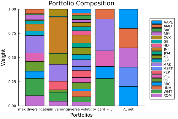
This page was generated using Literate.jl.