The source files can be found in examples/.
Entropy pooling
Black–Litterman blends views into the mean through a Gaussian update. Entropy pooling is more general in two ways. First, it expresses views as constraints on any moment — mean, variance, CVaR, skewness, kurtosis, even individual covariances and correlations. Second, it does not assume normality: it reweights the empirical scenarios so that the new distribution satisfies your views while staying as close as possible (in relative entropy / Kullback–Leibler divergence) to the original. The output is a fully reweighted prior, not just a shifted mean.
This is the second page of the view-prior arc — Black–Litterman came first, and Opinion Pooling follows, combining several entropy-pooling views into one.
In PortfolioOptimisers, EntropyPoolingPrior accepts a separate LinearConstraintEstimator per quantity. Mind the naming: mu_views is the mean, sigma_views is the variance, var_views is the Value at Risk, cvar_views the Conditional VaR, evar_views the Entropic VaR and rlvar_views the Relativistic VaR (tail-risk views), sk_views/kt_views are skewness/kurtosis, and cov_views/rho_views target covariances/correlations. Each is a list of string constraints over the UniverseSets names.
Reach for entropy pooling when your views are richer than "the mean will be x": views on volatility, tail risk (CVaR), skewness, or the correlation between two assets, possibly several at once. It is also the right tool when you distrust the normality assumption baked into Black–Litterman, since it reweights the empirical scenarios directly. For a simple mean-only view, Black–Litterman is lighter; to combine several entropy-pooling opinions, see Opinion Pooling.
using PortfolioOptimisers, PrettyTablesmmtfmt = (v, i, j) -> begin if j == 1 return v else return isa(v, Number) ? "$(round(v*100, digits=4)) %" : v endend;resfmt = (v, i, j) -> begin if j == 1 return v else return isa(v, Number) ? "$(round(v*100, digits=3)) %" : v endend;1. ReturnsResult data
We use the same S&P 500 slice as the other examples.
using CSV, TimeSeries, DataFramesX = TimeArray(CSV.File(joinpath(@__DIR__, "..", "SP500.csv.gz")); timestamp = :Date)[(end - 252):end]rd = prices_to_returns(X)ReturnsResult
nx ┼ 20-element Vector{String}
X ┼ 252×20 Matrix{Float64}
nf ┼ nothing
F ┼ nothing
nb ┼ nothing
B ┼ nothing
ts ┼ 252-element Vector{Date}
iv ┼ nothing
ivpa ┼ nothing
pnl ┼ AssetPanel
│ pf ┼ Vector{AbstractPanelField}: AbstractPanelField[]
│ amsk ┼ 252×20 AllTrueMask
│ emsk ┴ 252×20 AllTrueMask
2. Naming assets and groups
As with Black–Litterman, views reference assets and groups by name through an UniverseSets.
sets = UniverseSets(; dict = Dict("nx" => rd.nx, "tech" => ["AAPL", "AMD", "MSFT"], "energy" => ["CVX"]))UniverseSets
xkey ┼ String: "nx"
uxkey ┼ String: "ux"
tfkey ┼ String: "nf"
utfkey ┼ String: "uf"
cfkey ┼ String: "ncf"
ucfkey ┼ String: "ucf"
nikey ┼ String: "ni"
dict ┴ Dict{String, Vector{String}}: Dict("tech" => ["AAPL", "AMD", "MSFT"], "energy" => ["CVX"], "nx" => ["AAPL", "AMD", "BAC", "BBY", "CVX", "GE", "HD", "JNJ", "JPM", "KO", "LLY", "MRK", "MSFT", "PEP", "PFE", "PG", "RRC", "UNH", "WMT", "XOM"])
3. Views on several moments
Entropy-pooling views are also plain strings, but they can target different quantities. Here we state a mean view (Apple returns 8 bps) via mu_views, a relative mean view (tech outperforms energy), and a variance view (pin Apple's variance) via sigma_views. The comparison operators a view accepts depend on the moment: mu_views, sigma_views, sk_views, kt_views, cov_views, rho_views, cvar_views, evar_views and rlvar_views take ==, >= and <=; var_views (VaR) takes only == and >=. An unsupported operator raises a ParseError listing the ones allowed for that view.
A significance level belongs to the view rather than to the estimator: the CVaR at 1% and at 10% are different statistics of the same series. So var_views, cvar_views, evar_views and rlvar_views each take a ValueatRiskView, a ConditionalValueatRiskView, an EntropicValueatRiskView or a RelativisticValueatRiskView — each pairing a group of view equations with the alpha it is read under — or a vector of them for views stated at several levels. A RelativisticValueatRiskView carries a second parameter of the same kind, kappa: RLVaR reduces to the EVaR as kappa approaches zero and rises towards the worst loss of the sample as it approaches one, so the group states both. A prior(...) reference inside a group resolves at that group's level, and at its kappa where the family has one.
A tail view is not a linear function of the posterior probabilities, so it needs auxiliary variables and therefore a JuMPEntropyPooling in opt. The alg field of a tail view group picks how each view is written; left at nothing each takes the cheapest formulation that expresses it exactly — LinearConditionalValueatRiskView, ConicEntropicValueatRiskView and ConicRelativisticValueatRiskView for a lower bound or an equality at or above the prior value, and IntegerConditionalValueatRiskView, GridEntropicValueatRiskView or GridRelativisticValueatRiskView otherwise, which need a mixed-integer conic solver. A view over several assets whose coefficients share one sign, such as a group, is a positive combination of the measures and takes the same dual formulations. A relative view, whose coefficients carry both signs, takes the integer formulation for CVaR, and SequentialEntropicValueatRiskView or SequentialRelativisticValueatRiskView for the other two measures, which re-solve a convex program a few times and need no integer variable. SequentialConditionalValueatRiskView offers CVaR the same route. For an EntropicValueatRiskView or a RelativisticValueatRiskView the alg field is also where the grid of dual variables and the big-M constant live, so one group can take its own GridEntropicValueatRiskView or GridRelativisticValueatRiskView. ValueatRiskView has no alg: a VaR view is linear in the posterior probabilities, so there is no formulation to choose.
mu_views = LinearConstraintEstimator(; val = ["AAPL == 0.0008", "tech >= energy"])sigma_views = LinearConstraintEstimator(; val = ["AAPL == 0.0003"])ep = EntropyPoolingPrior(; sets = sets, mu_views = mu_views, sigma_views = sigma_views)EntropyPoolingPrior
pe ┼ EmpiricalPrior
│ ce ┼ PortfolioOptimisersCovariance
│ │ ce ┼ Covariance
│ │ │ me ┼ SimpleExpectedReturns
│ │ │ │ w ┴ nothing
│ │ │ ce ┼ GeneralCovariance
│ │ │ │ ce ┼ SimpleCovariance: SimpleCovariance(true)
│ │ │ │ w ┴ nothing
│ │ │ alg ┼ FullMoment()
│ │ │ w ┴ nothing
│ │ mp ┼ MatrixProcessing
│ │ │ pdm ┼ Posdef
│ │ │ │ alg ┼ UnionAll: NearestCorrelationMatrix.Newton
│ │ │ │ kwargs ┴ @NamedTuple{}: NamedTuple()
│ │ │ dn ┼ nothing
│ │ │ dt ┼ nothing
│ │ │ alg ┼ nothing
│ │ │ order ┴ NTuple{4, Symbol}: (:pdm, :dn, :dt, :alg)
│ me ┼ SimpleExpectedReturns
│ │ w ┴ nothing
│ horizon ┼ nothing
│ fill_limit ┴ nothing
mu_views ┼ LinearConstraintEstimator
│ val ┼ Vector{String}: ["AAPL == 0.0008", "tech >= energy"]
│ key ┴ nothing
var_views ┼ nothing
cvar_views ┼ nothing
evar_views ┼ nothing
rlvar_views ┼ nothing
sigma_views ┼ LinearConstraintEstimator
│ val ┼ Vector{String}: ["AAPL == 0.0003"]
│ key ┴ nothing
sk_views ┼ nothing
kt_views ┼ nothing
cov_views ┼ nothing
rho_views ┼ nothing
sets ┼ UniverseSets
│ xkey ┼ String: "nx"
│ uxkey ┼ String: "ux"
│ tfkey ┼ String: "nf"
│ utfkey ┼ String: "uf"
│ cfkey ┼ String: "ncf"
│ ucfkey ┼ String: "ucf"
│ nikey ┼ String: "ni"
│ dict ┴ Dict{String, Vector{String}}: Dict("tech" => ["AAPL", "AMD", "MSFT"], "energy" => ["CVX"], "nx" => ["AAPL", "AMD", "BAC", "BBY", "CVX", "GE", "HD", "JNJ", "JPM", "KO", "LLY", "MRK", "MSFT", "PEP", "PFE", "PG", "RRC", "UNH", "WMT", "XOM"])
opt ┼ OptimEntropyPooling
│ args ┼ Tuple{}: ()
│ kwargs ┼ @NamedTuple{}: NamedTuple()
│ sc1 ┼ Int64: 1
│ sc2 ┼ Float64: 1000.0
│ alg ┼ ExpEntropyPooling()
│ err ┴ nothing
w ┼ nothing
alg ┴ H1_EntropyPooling()
4. Prior vs reweighted posterior
We compute the entropy-pooling posterior and compare both the mean and the variance of Apple against the plain empirical prior — the mean view lifts the expected return while the variance view tightens the dispersion, exactly as instructed.
pr_ep = prior(ep, rd)pr_emp = prior(EmpiricalPrior(), rd)i_aapl = findfirst(==("AAPL"), rd.nx)pretty_table(DataFrame(["moment" => ["mean (AAPL)", "variance (AAPL)"], "Empirical" => [pr_emp.mu[i_aapl], pr_emp.sigma[i_aapl, i_aapl]], "Entropy pooling" => [pr_ep.mu[i_aapl], pr_ep.sigma[i_aapl, i_aapl]]]); formatters = [mmtfmt], title = "Apple moments: empirical vs entropy-pooling view")Apple moments: empirical vs entropy-pooling view
┌─────────────────┬───────────┬─────────────────┐
│ moment │ Empirical │ Entropy pooling │
│ String │ Float64 │ Float64 │
├─────────────────┼───────────┼─────────────────┤
│ mean (AAPL) │ -0.1126 % │ 0.08 % │
│ variance (AAPL) │ 0.05 % │ 0.0301 % │
└─────────────────┴───────────┴─────────────────┘The full expected-returns vectors, side by side.
pretty_table(DataFrame(["Assets" => rd.nx, "Empirical" => pr_emp.mu, "Entropy pooling" => pr_ep.mu]); formatters = [mmtfmt], title = "Expected returns: empirical vs entropy-pooling posterior")Expected returns: empirical vs entropy-pooling posterior
┌────────┬───────────┬─────────────────┐
│ Assets │ Empirical │ Entropy pooling │
│ String │ Float64 │ Float64 │
├────────┼───────────┼─────────────────┤
│ AAPL │ -0.1126 % │ 0.08 % │
│ AMD │ -0.2809 % │ 0.0698 % │
│ BAC │ -0.0934 % │ -0.0124 % │
│ BBY │ -0.0279 % │ 0.1921 % │
│ CVX │ 0.1945 % │ 0.243 % │
│ GE │ -0.0339 % │ 0.1278 % │
│ HD │ -0.0707 % │ 0.0504 % │
│ JNJ │ 0.0307 % │ 0.0766 % │
│ JPM │ -0.0417 % │ 0.0256 % │
│ KO │ 0.0497 % │ 0.098 % │
│ LLY │ 0.1305 % │ 0.1942 % │
│ MRK │ 0.1669 % │ 0.1861 % │
│ MSFT │ -0.1206 % │ 0.0932 % │
│ PEP │ 0.039 % │ 0.1159 % │
│ PFE │ -0.0256 % │ 0.033 % │
│ PG │ -0.0081 % │ 0.0576 % │
│ RRC │ 0.1824 % │ 0.2808 % │
│ UNH │ 0.0364 % │ 0.1196 % │
│ WMT │ 0.0163 % │ 0.0763 % │
│ XOM │ 0.2637 % │ 0.3058 % │
└────────┴───────────┴─────────────────┘Entropy-pooling posterior expected returns.
using StatsPlots, GraphRecipesplot_mu(pr_ep, rd.nx)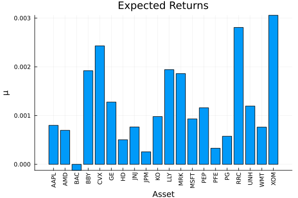
5. A tail view: relativistic value at risk
rlvar_views states a view on the relativistic VaR, the $\kappa$-deformed generalisation of the entropic VaR. Two numbers name the statistic. alpha is the significance level, and kappa is the deformation: RLVaR reduces to the EVaR as kappa approaches zero, and rises towards the worst loss of the sample as it approaches one. Both belong to the RelativisticValueatRiskView group rather than to the estimator.
That second number sets the first trap. No reweighting of the sample can push a tail measure past the worst loss the sample holds, so the room a lower-bound view has is whatever lies between the prior value and that loss. At kappa = 0.3 the RLVaR already sits near it, where the CVaR of the same asset does not.
Every field that takes a Solver also takes a vector of them, tried in order until one answers. Near the worst loss that spare matters. One configuration alone stops short when it reads the RLVaR of the posterior the <= view below produces, and says so. A second one with a shorter step answers it.
using Clarabel, HiGHS, Pajarito, JuMPslv = [Solver(; name = :clarabel1, solver = Clarabel.Optimizer, settings = Dict("verbose" => false), check_sol = (; allow_local = true, allow_almost = true)), Solver(; name = :clarabel2, solver = Clarabel.Optimizer, settings = Dict("verbose" => false, "max_step_fraction" => 0.85), check_sol = (; allow_local = true, allow_almost = true))]x_aapl = rd.X[:, i_aapl]rlvar_of = w -> RelativisticValueatRisk(; alpha = 0.05, kappa = 0.3, slv = slv, w = w)(x_aapl)prior_cvar = ConditionalValueatRisk(; alpha = 0.05)(x_aapl)prior_evar = EntropicValueatRisk(; alpha = 0.05, slv = slv)(x_aapl)prior_rlvar = RelativisticValueatRisk(; alpha = 0.05, kappa = 0.3, slv = slv)(x_aapl)worst_loss = maximum(-x_aapl)pretty_table(DataFrame(["Statistic" => ["CVaR", "EVaR", "RLVaR, kappa = 0.3", "worst loss"], "AAPL, prior" => [prior_cvar, prior_evar, prior_rlvar, worst_loss]]); formatters = [mmtfmt], title = "How much room a lower-bound tail view has")How much room a lower-bound tail view has
┌────────────────────┬─────────────┐
│ Statistic │ AAPL, prior │
│ String │ Float64 │
├────────────────────┼─────────────┤
│ CVaR │ 4.5734 % │
│ EVaR │ 5.0997 % │
│ RLVaR, kappa = 0.3 │ 5.3581 % │
│ worst loss │ 5.8684 % │
└────────────────────┴─────────────┘So "AAPL >= 1.25*prior(AAPL)" — a routine ask on cvar_views — is refused here with a DomainError naming that worst loss. A multiple near 1.05 is what this statistic affords.
A target below the prior is the other half, and it needs the other formulation. ConicRelativisticValueatRiskView bounds the RLVaR from below only, so a <= view takes GridRelativisticValueatRiskView instead. The grid picks one of its points with a binary vector, so it needs a solver for mixed-integer conic programs. Pajarito supplies one, driving HiGHS on the outer approximation and Clarabel on the cones. SequentialRelativisticValueatRiskView is the other route to a <= view: it bounds the RLVaR from above by a row that is linear in the posterior probabilities, and re-solves with the row re-read at each posterior until it is tight, so it needs no integer variable.
mip_slv = Solver(; name = :pajarito1, solver = optimizer_with_attributes(Pajarito.Optimizer, "verbose" => false, "oa_solver" => optimizer_with_attributes(HiGHS.Optimizer, JuMP.MOI.Silent() => true), "conic_solver" => optimizer_with_attributes(Clarabel.Optimizer, "verbose" => false)), check_sol = (; allow_local = true, allow_almost = true))lo_view = RelativisticValueatRiskView(; views = LinearConstraintEstimator(; val = "AAPL >= 1.05*prior(AAPL)"))hi_view = RelativisticValueatRiskView(; views = LinearConstraintEstimator(; val = "AAPL <= 0.95*prior(AAPL)"))pr_lo = prior(EntropyPoolingPrior(; sets = sets, opt = JuMPEntropyPooling(; slv = slv), rlvar_views = lo_view), rd)pr_hi = prior(EntropyPoolingPrior(; sets = sets, opt = JuMPEntropyPooling(; slv = mip_slv), rlvar_views = hi_view), rd)LowOrderPrior
X ┼ 252×20 Matrix{Float64}
o_X ┼ nothing
mu ┼ 20-element Vector{Float64}
sigma ┼ 20×20 Matrix{Float64}
chol ┼ nothing
w ┼ 252-element ProbabilityWeights{Float64, Float64, Vector{Float64}}
ens ┼ Float64: 251.28179039406996
kld ┼ Float64: 0.00285410721062299
ow ┼ nothing
rr ┼ nothing
fpr ┴ nothing
Each view lands on its target. The divergence column is the price it pays. The <= view is the cheaper of the two: to take 5% off a statistic that already sits near the worst loss is a smaller ask than to add 5% to it.
kldfmt = (v, i, j) -> begin if j == 1 return v elseif j == 2 return "$(round(v * 100, digits = 4)) %" else return isa(v, Number) ? string(round(v; sigdigits = 4)) : v endend;pretty_table(DataFrame(["Prior" => ["empirical", "RLVaR >= 1.05 prior, conic", "RLVaR <= 0.95 prior, grid"], "AAPL RLVaR" => [prior_rlvar, rlvar_of(pr_lo.w), rlvar_of(pr_hi.w)], "Divergence" => ["", pr_lo.kld, pr_hi.kld]]); formatters = [kldfmt], title = "Each RLVaR view lands on its target") Each RLVaR view lands on its target
┌────────────────────────────┬────────────┬────────────┐
│ Prior │ AAPL RLVaR │ Divergence │
│ String │ Float64 │ Any │
├────────────────────────────┼────────────┼────────────┤
│ empirical │ 5.3581 % │ │
│ RLVaR >= 1.05 prior, conic │ 5.626 % │ 0.007359 │
│ RLVaR <= 0.95 prior, grid │ 5.0902 % │ 0.002854 │
└────────────────────────────┴────────────┴────────────┘ConicRelativisticValueatRiskView writes $2T$ power cones. A longer sample, a smaller alpha, a smaller kappa, or two such views in one model can make a conic solver stop short of a solution. Give opt a vector of solver configurations, shorten the sample, or state the view under GridRelativisticValueatRiskView, whose lower-bound rows are linear in the posterior probabilities and write no cone at all.
6. Why it matters: views change the portfolio
Feeding the reweighted prior to a return-seeking optimiser tilts the portfolio toward the view-favoured assets, just as Black–Litterman did — but here the whole distribution, not only the mean, has been updated.
rf = 4.2 / 100 / 252res_emp = optimise(MeanRisk(; obj = MaximumRatio(; rf = rf), opt = JuMPOptimiser(; pe = pr_emp, slv = slv)))res_ep = optimise(MeanRisk(; obj = MaximumRatio(; rf = rf), opt = JuMPOptimiser(; pe = pr_ep, slv = slv)))pretty_table(DataFrame(["Assets" => rd.nx, "Empirical" => res_emp.w, "Entropy pooling" => res_ep.w]); formatters = [resfmt], title = "Maximum-ratio weights: empirical vs entropy pooling")Maximum-ratio weights: empirical vs entropy pooling
┌────────┬───────────┬─────────────────┐
│ Assets │ Empirical │ Entropy pooling │
│ String │ Float64 │ Float64 │
├────────┼───────────┼─────────────────┤
│ AAPL │ 0.0 % │ 0.0 % │
│ AMD │ 0.0 % │ 0.0 % │
│ BAC │ 0.0 % │ 0.0 % │
│ BBY │ 0.0 % │ 6.52 % │
│ CVX │ 0.0 % │ 0.0 % │
│ GE │ 0.0 % │ 0.0 % │
│ HD │ 0.0 % │ 0.0 % │
│ JNJ │ 0.0 % │ 0.0 % │
│ JPM │ 0.0 % │ 0.0 % │
│ KO │ 0.0 % │ 0.0 % │
│ LLY │ 0.002 % │ 6.913 % │
│ MRK │ 65.977 % │ 44.433 % │
│ MSFT │ 0.0 % │ 0.0 % │
│ PEP │ 0.0 % │ 12.545 % │
│ PFE │ 0.0 % │ 0.0 % │
│ PG │ 0.0 % │ 0.0 % │
│ RRC │ 0.0 % │ 0.0 % │
│ UNH │ 0.0 % │ 0.0 % │
│ WMT │ 0.0 % │ 0.0 % │
│ XOM │ 34.02 % │ 29.59 % │
└────────┴───────────┴─────────────────┘The composition plot makes the tilt visible.
plot_stacked_bar_composition([res_emp, res_ep], rd; xticks = (1:2, ["Empirical", "Entropy pooling"]))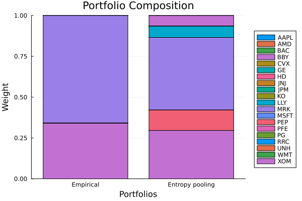
This page was generated using Literate.jl.