The source files can be found in examples/.
Clustering on a fundamentals panel
Feature matrices as a distance source builds its panel from a classification. That panel holds one named quantity per asset for each level of the classification, and each named quantity is a field. A fundamentals table is the harder case. It holds one row per asset and one column per reported quantity, it arrives with gaps, and its columns run over ranges that differ by orders of magnitude.
This page takes such a table from the raw numbers to a backtest. You build an AssetPanel with asset_panel, name the fields to cluster on with a FeatureDistance, and run HierarchicalRiskParity under a cross-validation. A classification raises none of the three questions that come up on the way.
- Blanks. A table with gaps needs a fill policy, and which policies you may use depends on whether the field carries an observation axis.
- Scale. The panel stores what you give it. A distance over columns on different scales reads the largest column and little else, so you standardise the table yourself, before you build the panel.
- What was reported at all. The fill records which cells held a value, and the selector can put that record into the matrix as a feature of its own.
The fundamentals below are written by hand. They have the shape of a real table and its awkwardness: mixed scales and a few gaps. They are not vendor data, and nothing follows from them about these companies.
using PortfolioOptimisers, CSV, TimeSeries, DataFrames, PrettyTables, Clarabel, StatsPlots, Statistics, LinearAlgebra, Clustering1. The universe and the table
We use the same twenty S&P 500 stocks as the other optimiser examples, over five years so that the backtests of sections 7 and 8 have room for their folds. The table holds five reported quantities per asset: log market capitalisation, book-to-price, gross profitability, leverage and dividend yield. NaN marks a cell the table does not carry.
X = TimeArray(CSV.File(joinpath(@__DIR__, "..", "SP500.csv.gz")); timestamp = :Date)[(end - 1260):end]rd0 = prices_to_returns(X)slv = Solver(; name = :clarabel, solver = Clarabel.Optimizer, settings = Dict("verbose" => false), check_sol = (; allow_local = true, allow_almost = true))sector = Dict("AAPL" => "Technology", "AMD" => "Technology", "MSFT" => "Technology", "BAC" => "Financials", "JPM" => "Financials", "CVX" => "Energy", "XOM" => "Energy", "RRC" => "Energy", "GE" => "Industrials", "BBY" => "ConsumerDiscretionary", "HD" => "ConsumerDiscretionary", "KO" => "ConsumerStaples", "PEP" => "ConsumerStaples", "PG" => "ConsumerStaples", "WMT" => "ConsumerStaples", "JNJ" => "HealthCare", "LLY" => "HealthCare", "MRK" => "HealthCare", "PFE" => "HealthCare", "UNH" => "HealthCare")fundamentals = DataFrame("Asset" => ["AAPL", "AMD", "BAC", "BBY", "CVX", "GE", "HD", "JNJ", "JPM", "KO", "LLY", "MRK", "MSFT", "PEP", "PFE", "PG", "RRC", "UNH", "WMT", "XOM"], "log_mcap" => [14.7, 11.8, 12.5, 10.1, 12.6, 12.0, 12.7, 13.0, 13.1, 12.4, 13.2, 12.5, 14.6, 12.3, 12.1, 12.7, 9.2, 13.0, 13.1, 12.9], "book_to_price" => [0.05, 0.08, 0.95, 0.31, 0.62, 0.28, 0.02, 0.19, 0.78, 0.11, 0.06, 0.14, 0.06, 0.09, 0.27, 0.10, 1.42, 0.13, 0.21, 0.55], "gross_profitability" => [0.44, 0.21, 0.11, 0.09, 0.34, 0.16, 0.38, 0.32, 0.51, 0.29, 0.47, 0.36, 0.49, 0.26, 0.30, 0.33, NaN, 0.23, 0.13, 0.19], "leverage" => [1.71, 0.29, 5.90, 1.20, 0.55, 2.90, 8.10, 0.83, 6.40, 1.60, 0.72, 0.94, 0.42, 2.20, 0.61, 1.30, NaN, 0.88, 1.05, 0.48], "dividend_yield" => [0.005, NaN, 0.024, 0.041, 0.038, 0.003, 0.023, 0.029, 0.007, 0.030, 0.010, 0.026, 0.008, 0.027, 0.043, 0.024, NaN, 0.013, 0.015, 0.034])pretty_table(fundamentals; formatters = [(v, i, j) -> isa(v, AbstractFloat) ? round(v; digits = 4) : v], title = "The reported table, gaps included") The reported table, gaps included
┌────────┬──────────┬───────────────┬─────────────────────┬──────────┬────────────────┐
│ Asset │ log_mcap │ book_to_price │ gross_profitability │ leverage │ dividend_yield │
│ String │ Float64 │ Float64 │ Float64 │ Float64 │ Float64 │
├────────┼──────────┼───────────────┼─────────────────────┼──────────┼────────────────┤
│ AAPL │ 14.7 │ 0.05 │ 0.44 │ 1.71 │ 0.005 │
│ AMD │ 11.8 │ 0.08 │ 0.21 │ 0.29 │ NaN │
│ BAC │ 12.5 │ 0.95 │ 0.11 │ 5.9 │ 0.024 │
│ BBY │ 10.1 │ 0.31 │ 0.09 │ 1.2 │ 0.041 │
│ CVX │ 12.6 │ 0.62 │ 0.34 │ 0.55 │ 0.038 │
│ GE │ 12.0 │ 0.28 │ 0.16 │ 2.9 │ 0.003 │
│ HD │ 12.7 │ 0.02 │ 0.38 │ 8.1 │ 0.023 │
│ JNJ │ 13.0 │ 0.19 │ 0.32 │ 0.83 │ 0.029 │
│ JPM │ 13.1 │ 0.78 │ 0.51 │ 6.4 │ 0.007 │
│ KO │ 12.4 │ 0.11 │ 0.29 │ 1.6 │ 0.03 │
│ LLY │ 13.2 │ 0.06 │ 0.47 │ 0.72 │ 0.01 │
│ MRK │ 12.5 │ 0.14 │ 0.36 │ 0.94 │ 0.026 │
│ MSFT │ 14.6 │ 0.06 │ 0.49 │ 0.42 │ 0.008 │
│ PEP │ 12.3 │ 0.09 │ 0.26 │ 2.2 │ 0.027 │
│ PFE │ 12.1 │ 0.27 │ 0.3 │ 0.61 │ 0.043 │
│ PG │ 12.7 │ 0.1 │ 0.33 │ 1.3 │ 0.024 │
│ RRC │ 9.2 │ 1.42 │ NaN │ NaN │ NaN │
│ UNH │ 13.0 │ 0.13 │ 0.23 │ 0.88 │ 0.013 │
│ WMT │ 13.1 │ 0.21 │ 0.13 │ 1.05 │ 0.015 │
│ XOM │ 12.9 │ 0.55 │ 0.19 │ 0.48 │ 0.034 │
└────────┴──────────┴───────────────┴─────────────────────┴──────────┴────────────────┘This table lists the assets in the order of the returns, but a table from another source can use another order. The panel reads a row by its position, and it never reads the name. So put the table into the order of rd0.nx once, in the cell below, and do not assume that the two orders match.
row_of = Dict(a => i for (i, a) in pairs(fundamentals.Asset))order = [row_of[a] for a in rd0.nx]tbl = fundamentals[order, :]println("The table is aligned to the returns: ", tbl.Asset == rd0.nx)The table is aligned to the returns: true2. You standardise the table before you build the panel
An AssetPanel stores what you give it. asset_panel does not standardise a field, and that is a decision rather than a gap. The right transform follows from what the column holds, and a level, a ratio, a rank and a logarithm each ask for a different one. The panel builder does not guess which you have.
It matters here because the default AngularDist does not change when you rescale the whole row of an asset, and it does change when you rescale one column. Stack the five columns without standardising them, and log_mcap is the largest entry of every row, so every row points mostly along the log_mcap axis. A difference in log_mcap between two assets then changes the length of a row more than its direction. The angle between two rows comes mostly from leverage, the column with the widest spread, and the three columns that stay under 1.5 count for much less.
raw_fields = ["log_mcap", "book_to_price", "gross_profitability", "leverage", "dividend_yield"]pretty_table(DataFrame("Field" => raw_fields, "Smallest" => [minimum(filter(!isnan, tbl[!, f])) for f in raw_fields], "Largest" => [maximum(filter(!isnan, tbl[!, f])) for f in raw_fields], "Standard deviation" => [std(filter(!isnan, tbl[!, f])) for f in raw_fields]); formatters = [(v, i, j) -> isa(v, AbstractFloat) ? round(v; digits = 4) : v], title = "Range and standard deviation of the five columns") Range and standard deviation of the five columns
┌─────────────────────┬──────────┬─────────┬────────────────────┐
│ Field │ Smallest │ Largest │ Standard deviation │
│ String │ Float64 │ Float64 │ Float64 │
├─────────────────────┼──────────┼─────────┼────────────────────┤
│ log_mcap │ 9.2 │ 14.7 │ 1.2311 │
│ book_to_price │ 0.02 │ 1.42 │ 0.3674 │
│ gross_profitability │ 0.09 │ 0.51 │ 0.1284 │
│ leverage │ 0.29 │ 8.1 │ 2.2615 │
│ dividend_yield │ 0.003 │ 0.043 │ 0.0126 │
└─────────────────────┴──────────┴─────────┴────────────────────┘The usual transform for a table of this shape is a z-score down each column, over the cells that hold a value. The blanks stay blank. Standardising a column does not fill it, and the fill policy is the next decision, one step later.
function zscore_column(v) obs = filter(!isnan, v) m, s = mean(obs), std(obs) return [isnan(x) ? NaN : (x - m) / s for x in v]endzfields = Dict(f => zscore_column(tbl[!, f]) for f in raw_fields)Dict{String, Vector{Float64}} with 5 entries:
"log_mcap" => [1.76668, -0.588894, -0.0203067, -1.96975, 0.0609201, -0.426441, 0.142147, 0.385827, 0.467054, -0.101534, 0.548281, -0.0203067, 1.68546, -0.18276, -0.345214, 0.142147, -2.70079, 0.385827, 0.467054, 0.304601]
"book_to_price" => [-0.737687, -0.656024, 1.71219, -0.029943, 0.813905, -0.111606, -0.819349, -0.356594, 1.24944, -0.574361, -0.710466, -0.492698, -0.710466, -0.628803, -0.138827, -0.601582, 2.99158, -0.519919, -0.302152, 0.623359]
"dividend_yield" => [-1.36427, NaN, 0.140828, 1.48749, 1.24985, -1.5227, 0.0616122, 0.536906, -1.20584, 0.616122, -0.968191, 0.299259, -1.12662, 0.378475, 1.64593, 0.140828, NaN, -0.730544, -0.572113, 0.932984]
"gross_profitability" => [1.12739, -0.664138, -1.44306, -1.59885, 0.348467, -1.0536, 0.660038, 0.192682, 1.67264, -0.0409962, 1.36107, 0.504253, 1.51686, -0.274674, 0.0368965, 0.270575, NaN, -0.508352, -1.28728, -0.819923]
"leverage" => [-0.130097, -0.758005, 1.72267, -0.355613, -0.643036, 0.396108, 2.69549, -0.519223, 1.94377, -0.178737, -0.567863, -0.470582, -0.70052, 0.0865759, -0.616504, -0.311394, NaN, -0.497113, -0.421941, -0.673989]3. Building the panel
asset_panel takes each field in its raw form, blanks and all, and returns the panel that a ReturnsResult then holds. A NumericPanelInput holds one reported quantity. panel_input reads the sector classification off a UniverseSets and returns a CategoricalPanelInput.
Every input takes a fill policy, and the default alg = nothing refuses a blank. That is the right default, because a blank that reaches the panel becomes a zero in the matrix, and a zero in a standardised column is the mean rather than a gap. The build asks you what a gap means instead.
The values here hold one number per asset and no observation axis, which makes this a static input. asset_panel refuses the two directional policies on such an input, because they carry a value along the observation axis, and there is none. A static table takes ConstantPanelFill, and after the z-score 0.0 is the mean over the assets.
sets = UniverseSets(; xkey = "nx", dict = Dict("nx" => rd0.nx, "nx_sector" => [sector[a] for a in rd0.nx]))inputs = [[NumericPanelInput(; name = f, vals = zfields[f], alg = ConstantPanelFill(; val = 0.0)) for f in raw_fields]; panel_input(sets, "nx_sector")]pnl = asset_panel(inputs)directional_refusal = try asset_panel([NumericPanelInput(; name = "log_mcap", vals = zfields["log_mcap"], alg = ForwardPanelFill())]) "no error"catch err sprint(showerror, err)endprintln(directional_refusal)ArgumentError: the Panel Field "log_mcap" is static, so it has no observation axis to carry a value along, and its fill policy ForwardPanelFill is directional. Use alg = nothing or ConstantPanelFill, or give the raw values an observation axis.4. What the panel holds
The panel is static. Every field holds one value per asset and no field records anything over time. feature_matrix stacks the panel into a matrix of assets by features, and feature_labels names its columns. There is one column per numeric field and one per level of the categorical field.
Z = feature_matrix(pnl)nz = feature_labels(pnl)pretty_table(DataFrame("Field" => [f.name for f in pnl.pf], "Kind" => [string(nameof(typeof(f))) for f in pnl.pf], "Columns it contributes" => [count(l -> first(l) == f.name || l == f.name, nz) for f in pnl.pf]); title = "Six fields, $(size(Z, 2)) feature columns")println("Static panel: ", PortfolioOptimisers.panel_is_static(pnl))println("The labels rebuild the matrix: ", feature_matrix(pnl, nz) == Z) Six fields, 12 feature columns
┌─────────────────────┬───────────────────────┬────────────────────────┐
│ Field │ Kind │ Columns it contributes │
│ String │ String │ Int64 │
├─────────────────────┼───────────────────────┼────────────────────────┤
│ log_mcap │ NumericPanelField │ 1 │
│ book_to_price │ NumericPanelField │ 1 │
│ gross_profitability │ NumericPanelField │ 1 │
│ leverage │ NumericPanelField │ 1 │
│ dividend_yield │ NumericPanelField │ 1 │
│ sector │ CategoricalPanelField │ 7 │
└─────────────────────┴───────────────────────┴────────────────────────┘
Static panel: true
The labels rebuild the matrix: true5. Clustering on named fields
sel on the FeatureDistance names the fields to stack. The panel names its own fields, so you write the names rather than count columns. ["book_to_price", "gross_profitability"] gives a hierarchy built on value and quality, ["sector"] gives the classification, and nothing gives every field the panel holds.
The panel is data and the selector is a setting, so the six runs below read one panel.
rd = ReturnsResult(; nx = rd0.nx, X = rd0.X, ts = rd0.ts, pnl = pnl)onc = OptimalNumberClusters(; alg = 4)hierarchies = ["Correlation (no panel)" => nothing, "Every field" => FeatureDistance(), "Sector only" => FeatureDistance(; sel = ["sector"]), "Value and quality" => FeatureDistance(; sel = ["book_to_price", "gross_profitability"]), "Size and leverage" => FeatureDistance(; sel = ["log_mcap", "leverage"]), "Sector, then value" => FeatureDistance(; sel = ["sector", "book_to_price"])]cut_rows = DataFrame()cuts = Dict{String, Vector{Int}}()for (hname, de) in hierarchies cle = if isnothing(de) ClustersEstimator(; onc = onc) else ClustersEstimator(; de = de, onc = onc) end clr = clusterise(cle, rd) cuts[hname] = cutree(clr.res; k = 4) append!(cut_rows, DataFrame("Hierarchy" => hname, "Feature columns" => if isnothing(de) 0 else size(feature_matrix(de, nothing, rd, rd.X), 2) end, "Clusters chosen" => clr.k, "ARI against correlation" => round(randindex(cuts["Correlation (no panel)"], cuts[hname])[1]; digits = 3)))endpretty_table(cut_rows; title = "Six hierarchies, scored against the correlation cut") Six hierarchies, scored against the correlation cut
┌────────────────────────┬─────────────────┬─────────────────┬─────────────────────────┐
│ Hierarchy │ Feature columns │ Clusters chosen │ ARI against correlation │
│ String │ Int64 │ Int64 │ Float64 │
├────────────────────────┼─────────────────┼─────────────────┼─────────────────────────┤
│ Correlation (no panel) │ 0 │ 4 │ 1.0 │
│ Every field │ 12 │ 4 │ 0.222 │
│ Sector only │ 7 │ 4 │ 0.646 │
│ Value and quality │ 2 │ 4 │ 0.173 │
│ Size and leverage │ 2 │ 4 │ -0.063 │
│ Sector, then value │ 8 │ 4 │ 0.844 │
└────────────────────────┴─────────────────┴─────────────────┴─────────────────────────┘The last column scores each cut against the cut the correlations give, where 1 means the two cuts are the same. A hierarchy built on value and one built on size each score low against the correlations. That is a reason to reach for a panel, because each one answers a question the price history does not hold.
The next table prints the four-way cuts themselves, one column per hierarchy.
pretty_table(DataFrame(["Asset" => rd.nx; "Sector" => [sector[a] for a in rd.nx]; [hname => cuts[hname] for (hname, _) in hierarchies]...]); title = "Four-cluster cuts, one column per hierarchy") Four-cluster cuts, one column per hierarchy
┌────────┬───────────────────────┬────────────────────────┬─────────────┬─────────────┬───────────────────┬───────────────────┬────────────────────┐
│ Asset │ Sector │ Correlation (no panel) │ Every field │ Sector only │ Value and quality │ Size and leverage │ Sector, then value │
│ String │ String │ Int64 │ Int64 │ Int64 │ Int64 │ Int64 │ Int64 │
├────────┼───────────────────────┼────────────────────────┼─────────────┼─────────────┼───────────────────┼───────────────────┼────────────────────┤
│ AAPL │ Technology │ 1 │ 1 │ 1 │ 1 │ 1 │ 1 │
│ AMD │ Technology │ 1 │ 2 │ 1 │ 2 │ 2 │ 1 │
│ BAC │ Financials │ 2 │ 3 │ 1 │ 3 │ 3 │ 2 │
│ BBY │ ConsumerDiscretionary │ 1 │ 2 │ 1 │ 3 │ 4 │ 1 │
│ CVX │ Energy │ 2 │ 3 │ 2 │ 4 │ 2 │ 2 │
│ GE │ Industrials │ 2 │ 2 │ 1 │ 3 │ 4 │ 1 │
│ HD │ ConsumerDiscretionary │ 1 │ 1 │ 1 │ 1 │ 3 │ 1 │
│ JNJ │ HealthCare │ 3 │ 4 │ 3 │ 1 │ 1 │ 3 │
│ JPM │ Financials │ 2 │ 1 │ 1 │ 4 │ 3 │ 2 │
│ KO │ ConsumerStaples │ 4 │ 4 │ 4 │ 2 │ 2 │ 4 │
│ LLY │ HealthCare │ 3 │ 1 │ 3 │ 1 │ 1 │ 3 │
│ MRK │ HealthCare │ 3 │ 4 │ 3 │ 1 │ 2 │ 3 │
│ MSFT │ Technology │ 1 │ 1 │ 1 │ 1 │ 1 │ 1 │
│ PEP │ ConsumerStaples │ 4 │ 4 │ 4 │ 2 │ 4 │ 4 │
│ PFE │ HealthCare │ 3 │ 4 │ 3 │ 1 │ 2 │ 3 │
│ PG │ ConsumerStaples │ 4 │ 4 │ 4 │ 1 │ 1 │ 4 │
│ RRC │ Energy │ 2 │ 3 │ 2 │ 4 │ 4 │ 2 │
│ UNH │ HealthCare │ 3 │ 2 │ 3 │ 2 │ 1 │ 3 │
│ WMT │ ConsumerStaples │ 4 │ 2 │ 4 │ 3 │ 1 │ 4 │
│ XOM │ Energy │ 2 │ 3 │ 2 │ 3 │ 1 │ 2 │
└────────┴───────────────────────┴────────────────────────┴─────────────┴─────────────┴───────────────────┴───────────────────┴────────────────────┘6. The observed mask is a feature
The fill removed the blanks and recorded which cells held a value. Write "name" => :observed in the selector and that record enters the matrix as one column of zeros and ones. On a table with many gaps, whether a quantity was reported can separate the assets more sharply than the number reported, and it costs one entry in the selector.
leverage and gross_profitability each hold one gap here, and dividend_yield holds two.
obs_rows = DataFrame()for f in raw_fields m = feature_matrix(pnl, [f => :observed]) append!(obs_rows, DataFrame("Field" => f, "Reported" => Int(sum(m)), "Missing" => Int(length(m) - sum(m))))endpretty_table(obs_rows; title = "Reported and missing cells by field")de_reported = FeatureDistance(; sel = ["book_to_price", "gross_profitability", "gross_profitability" => :observed, "dividend_yield" => :observed])println("The selector's own labels: ", feature_labels(de_reported, nothing, rd, rd.X)) Reported and missing cells by field
┌─────────────────────┬──────────┬─────────┐
│ Field │ Reported │ Missing │
│ String │ Int64 │ Int64 │
├─────────────────────┼──────────┼─────────┤
│ log_mcap │ 20 │ 0 │
│ book_to_price │ 20 │ 0 │
│ gross_profitability │ 19 │ 1 │
│ leverage │ 19 │ 1 │
│ dividend_yield │ 18 │ 2 │
└─────────────────────┴──────────┴─────────┘
The selector's own labels: Any["book_to_price", "gross_profitability", "gross_profitability" => :observed, "dividend_yield" => :observed]An :observed entry on a field that held no blank gives a column of ones. The record is right, because nothing was missing. A column of ones adds the same amount to every dot product and to every squared norm, so it still moves the cosine between two rows. It changes the distances and tells you nothing about the assets, so leave it out.
7. Through a cross-validation
The panel changes nothing downstream. HierarchicalRiskParity takes the clustering estimator as it always does, and cross_val_predict runs it over the folds. We train on one year and rebalance every quarter.
A static panel carries no observation axis, so a fold has nothing to cut on it. The same twenty rows describe the universe in every window. That is what this route is for. Cross-validation fits both hierarchies again on every fold. The one built on the correlations changes with the window, and the one built on this panel comes out the same every time. Only the covariance that allocates inside it changes.
walk = IndexWalkForward(252, 63)function backtest(de) cle = if isnothing(de) ClustersEstimator(; onc = onc) else ClustersEstimator(; de = de, onc = onc) end return cross_val_predict(HierarchicalRiskParity(; opt = HierarchicalOptimiser(; pe = EmpiricalPrior(), cle = cle, slv = slv), r = Variance()), rd, walk)endfunction backtest_row(name, p) r = p.mrd.X turn = mean(abs, reduce(vcat, [p.pred[i + 1].res.w - p.pred[i].res.w for i in 1:(length(p.pred) - 1)])) return (; Hierarchy = name, var"Annual return" = mean(r) * 252, var"Annual volatility" = std(r) * sqrt(252), var"Sharpe ratio" = mean(r) / std(r) * sqrt(252), var"Maximum drawdown" = expected_risk(MaximumDrawdown(), p), var"Mean weight change" = turn)endbt = ["Correlation" => nothing, "Every field" => FeatureDistance(), "Sector only" => FeatureDistance(; sel = ["sector"]), "Value and quality" => FeatureDistance(; sel = ["book_to_price", "gross_profitability"])]results = [(name, backtest(de)) for (name, de) in bt]pretty_table(DataFrame([backtest_row(name, p) for (name, p) in results]); formatters = [(v, i, j) -> isa(v, AbstractFloat) ? round(v; digits = 4) : v], title = "Out-of-sample results over $(length(last(first(results)).pred)) quarterly rebalances") Out-of-sample results over 16 quarterly rebalances
┌───────────────────┬───────────────┬───────────────────┬──────────────┬──────────────────┬────────────────────┐
│ Hierarchy │ Annual return │ Annual volatility │ Sharpe ratio │ Maximum drawdown │ Mean weight change │
│ String │ Float64 │ Float64 │ Float64 │ Float64 │ Float64 │
├───────────────────┼───────────────┼───────────────────┼──────────────┼──────────────────┼────────────────────┤
│ Correlation │ 0.1943 │ 0.1972 │ 0.9855 │ 0.3033 │ 0.0123 │
│ Every field │ 0.1874 │ 0.1959 │ 0.957 │ 0.306 │ 0.0059 │
│ Sector only │ 0.1921 │ 0.1985 │ 0.9677 │ 0.3171 │ 0.0062 │
│ Value and quality │ 0.1877 │ 0.1982 │ 0.9473 │ 0.3122 │ 0.006 │
└───────────────────┴───────────────┴───────────────────┴──────────────┴──────────────────┴────────────────────┘Read the Mean weight change column. Each hierarchy built from the panel moves its weights less between rebalances than the one built from the correlations, because a table that does not change between folds gives a tree that does not change either.
plot_portfolio_cumulative_returns(last(results[2]))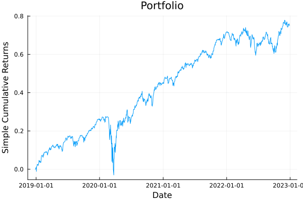
8. When the table does move
A fundamentals table that is restated over time is a time-varying input. Its values carry an observation axis, and a fold cuts that axis as it cuts the returns. The selector, the distance and the optimiser stay as they are. What changes is the shape of the array you pass NumericPanelInput, which gains a second dimension.
The observation axis brings two things with it.
ForwardPanelFillis now allowed, and it is the policy that is safe across a fold, because it only carries a value forward in time.- The
FeatureDistanceneeds a rule,alg, that turns the stack of periods into one distance matrix.
T, N = size(rd.X)drift = zeros(T, N)for t in 1:T, i in 1:N drift[t, i] = zfields["book_to_price"][i] + sum(view(rd.X, 1:t, i))enddrift[1:5, 1:2] .= NaNpnl_tv = asset_panel([NumericPanelInput(; name = "book_to_price", vals = drift, alg = ForwardPanelFill()), NumericPanelInput(; name = "log_mcap", vals = repeat(transpose(zfields["log_mcap"]), T), alg = ConstantPanelFill(; val = 0.0)), panel_input(sets, "nx_sector")])rd_tv = ReturnsResult(; nx = rd0.nx, X = rd0.X, ts = rd0.ts, pnl = pnl_tv)pretty_table(DataFrame("Panel" => ["Static (section 3)", "Time-varying (section 8)"], "Static?" => [PortfolioOptimisers.panel_is_static(pnl), PortfolioOptimisers.panel_is_static(pnl_tv)], "Feature matrix" => [string(size(feature_matrix(pnl))), string(size(feature_matrix(pnl_tv)))], "After a 100-row, 3-asset view" => [string(size(feature_matrix(PortfolioOptimisers.port_opt_view(rd, 1:100, [1, 2, 3]).pnl))), string(size(feature_matrix(PortfolioOptimisers.port_opt_view(rd_tv, 1:100, [1, 2, 3]).pnl)))]); title = "Shape of each panel before and after a view") Shape of each panel before and after a view
┌──────────────────────────┬─────────┬────────────────┬───────────────────────────────┐
│ Panel │ Static? │ Feature matrix │ After a 100-row, 3-asset view │
│ String │ Bool │ String │ String │
├──────────────────────────┼─────────┼────────────────┼───────────────────────────────┤
│ Static (section 3) │ true │ (20, 12) │ (3, 12) │
│ Time-varying (section 8) │ false │ (20, 9, 1260) │ (3, 9, 100) │
└──────────────────────────┴─────────┴────────────────┴───────────────────────────────┘Keeping the first 100 observations and the first three assets cut both panels to three assets, and only the time-varying panel also lost every observation after the hundredth. The static panel has no observation axis, so the observation half of the view leaves it whole. Which of the two shapes you want follows from your data rather than from the library.
The sector field of the time-varying panel is a static input among time-varying ones. asset_panel gives it the observation axis of the others and stores its values once.
We cluster the time-varying panel under each of the four collapse rules. Then we backtest it with the default rule, LastRow, against the every-field hierarchy on the static panel of section 7.
collapse_rows = DataFrame()for alg in (LastRow(), AggregateFeatures(), AggregateDistances(), StackObservations()) de = FeatureDistance(; alg = alg) clr = clusterise(ClustersEstimator(; de = de, onc = onc), rd_tv) append!(collapse_rows, DataFrame("Collapse" => string(nameof(typeof(alg))), "Clusters chosen" => clr.k, "Mean distance" => round(mean(clr.D); digits = 4), "ARI against correlation" => round(randindex(cuts["Correlation (no panel)"], cutree(clr.res; k = 4))[1]; digits = 3)))endpretty_table(collapse_rows; title = "One time-varying panel, four collapse rules")bt_tv = cross_val_predict(HierarchicalRiskParity(; opt = HierarchicalOptimiser(; pe = EmpiricalPrior(), cle = ClustersEstimator(; de = FeatureDistance(), onc = onc), slv = slv), r = Variance()), rd_tv, walk)pretty_table(DataFrame([backtest_row("Static panel", last(results[2])), backtest_row("Time-varying panel", bt_tv)]); formatters = [(v, i, j) -> isa(v, AbstractFloat) ? round(v; digits = 4) : v], title = "The same optimiser over the two panel shapes") One time-varying panel, four collapse rules
┌────────────────────┬─────────────────┬───────────────┬─────────────────────────┐
│ Collapse │ Clusters chosen │ Mean distance │ ARI against correlation │
│ String │ Int64 │ Float64 │ Float64 │
├────────────────────┼─────────────────┼───────────────┼─────────────────────────┤
│ LastRow │ 4 │ 0.3871 │ 0.549 │
│ AggregateFeatures │ 4 │ 0.4355 │ 0.527 │
│ AggregateDistances │ 4 │ 0.4278 │ 0.527 │
│ StackObservations │ 4 │ 0.4239 │ 0.527 │
└────────────────────┴─────────────────┴───────────────┴─────────────────────────┘
The same optimiser over the two panel shapes
┌────────────────────┬───────────────┬───────────────────┬──────────────┬──────────────────┬────────────────────┐
│ Hierarchy │ Annual return │ Annual volatility │ Sharpe ratio │ Maximum drawdown │ Mean weight change │
│ String │ Float64 │ Float64 │ Float64 │ Float64 │ Float64 │
├────────────────────┼───────────────┼───────────────────┼──────────────┼──────────────────┼────────────────────┤
│ Static panel │ 0.1874 │ 0.1959 │ 0.957 │ 0.306 │ 0.0059 │
│ Time-varying panel │ 0.1979 │ 0.1996 │ 0.9918 │ 0.3041 │ 0.0099 │
└────────────────────┴───────────────┴───────────────────┴──────────────┴──────────────────┴────────────────────┘The time-varying panel earns the higher ratio of the two here, and the last column is what it costs. It moves its weights more than twice as far between rebalances, because a table that is restated every day gives a tree that changes every fold. The two panels also hold different fields, so the shape of the input is not the only difference between the two rows.
9. Summary
asset_panelis where the panel is built. It takes the raw table, blanks and all, and returns theAssetPanelaReturnsResultholds.- A fill policy is compulsory. The default
alg = nothingrefuses a blank rather than let it become a zero in the matrix. A static input takesConstantPanelFill, and the two directional policies need an observation axis and are refused without one. - You standardise the table, before the panel is built. The default
AngularDistdoes not change when you rescale a row, and it does change when you rescale a column. selnames fields, so you write a hierarchy in the words of your own table. An:observedentry turns "was this reported" into a feature.- A fold does not cut a static panel. That is why a hierarchy built from fundamentals does not move between rebalances. A fold does cut a time-varying panel, and a time-varying panel needs a collapse rule.
ClustersEstimator,HierarchicalRiskParityandcross_val_predictare unchanged. The panel is data on the returns result, and the distance estimator is the only thing that reads it.
This page was generated using Literate.jl.