The source files can be found in examples/.
Example 7: Risk factor optimisation
This example shows how to use factor models to perform optimisations. These reduce the estimation error by modelling asset returns as a function of common risk factors.
using PortfolioOptimisers, PrettyTables
# Format for pretty tables.
tsfmt = (v, i, j) -> begin
    if j == 1
        return Date(v)
    else
        return v
    end
end;
resfmt = (v, i, j) -> begin
    if j == 1
        return v
    else
        return isa(v, Number) ? "$(round(v*100, digits=3)) %" : v
    end
end;
mmtfmt = (v, i, j) -> begin
    if i == j == 1
        return v
    else
        return isa(v, Number) ? "$(round(v*100, digits=3)) %" : v
    end
end;
hmmtfmt = (v, i, j) -> begin
    if i == j == 1
        return v
    else
        return isa(v, Number) ? "$(round(v*100*1e4, digits=2))e-4 %" : v
    end
end;
1. ReturnsResult data
We will use the same data as the previous example. But we will also load factor data.
using CSV, TimeSeries, DataFrames

X = TimeArray(CSV.File(joinpath(@__DIR__, "SP500.csv.gz")); timestamp = :Date)[(end - 252):end]
pretty_table(X[(end - 5):end]; formatters = [tsfmt])

F = TimeArray(CSV.File(joinpath(@__DIR__, "Factors.csv.gz")); timestamp = :Date)[(end - 252):end]
pretty_table(F[(end - 5):end]; formatters = [tsfmt])

# Compute the returns
rd = prices_to_returns(X, F)
ReturnsResult
nx ┼ 20-element Vector{String}
X ┼ 252×20 Matrix{Float64}
nf ┼ Vector{String}: ["MTUM", "QUAL", "SIZE", "USMV", "VLUE"]
F ┼ 252×5 Matrix{Float64}
nb ┼ nothing
B ┼ nothing
ts ┼ 252-element Vector{Date}
iv ┼ nothing
ivpa ┴ nothing2. Prior statistics
PortfolioOptimisers.jl supports a wide range of prior models. Here we will use four of them:
EmpiricalPrior: Computes the expected returns vector and covariance matrix from the empirical data.FactorPrior: Computes the expected returns vector and covariance matrix using a factor model.HighOrderPriorEstimator: Computes the expected returns vector and covariance matrix using the low order prior estimator provided, plus the coskewness and/or cokurtosis using the computed expected returns vector.HighOrderFactorPriorEstimator: Computes the expected returns vector and covariance matrix, plus the coskewness and/or cokurtosis using a factor model.
Priors whos names don't start with the prefix High return LowOrderPrior, while those that do return HighOrderPrior objects.
We have two different regression models with various targets. We won't explore them all in detail here, see StepwiseRegression and DimensionReductionRegression for details. First let's define the prior estimators.
pes = [EmpiricalPrior(),#
       FactorPrior(),#
       FactorPrior(; re = DimensionReductionRegression()),#
       HighOrderPriorEstimator(),#
       HighOrderPriorEstimator(; pe = FactorPrior()),#
       HighOrderPriorEstimator(; pe = FactorPrior(; re = DimensionReductionRegression())),#
       HighOrderFactorPriorEstimator(;),#
       HighOrderFactorPriorEstimator(;
                                     pe = FactorPrior(;
                                                      re = DimensionReductionRegression()))]
8-element Vector{AbstractPriorEstimator}:
EmpiricalPrior
ce ┼ PortfolioOptimisersCovariance
│ ce ┼ Covariance
│ │ me ┼ SimpleExpectedReturns
│ │ │ w ┴ nothing
│ │ ce ┼ GeneralCovariance
│ │ │ ce ┼ SimpleCovariance: SimpleCovariance(true)
│ │ │ w ┴ nothing
│ │ alg ┴ Full()
│ mp ┼ DenoiseDetoneAlgMatrixProcessing
│ │ pdm ┼ Posdef
│ │ │ alg ┼ UnionAll: NearestCorrelationMatrix.Newton
│ │ │ kwargs ┴ @NamedTuple{}: NamedTuple()
│ │ dn ┼ nothing
│ │ dt ┼ nothing
│ │ alg ┼ nothing
│ │ order ┴ DenoiseDetoneAlg()
me ┼ SimpleExpectedReturns
│ w ┴ nothing
horizon ┴ nothing
FactorPrior
pe ┼ EmpiricalPrior
│ ce ┼ PortfolioOptimisersCovariance
│ │ ce ┼ Covariance
│ │ │ me ┼ SimpleExpectedReturns
│ │ │ │ w ┴ nothing
│ │ │ ce ┼ GeneralCovariance
│ │ │ │ ce ┼ SimpleCovariance: SimpleCovariance(true)
│ │ │ │ w ┴ nothing
│ │ │ alg ┴ Full()
│ │ mp ┼ DenoiseDetoneAlgMatrixProcessing
│ │ │ pdm ┼ Posdef
│ │ │ │ alg ┼ UnionAll: NearestCorrelationMatrix.Newton
│ │ │ │ kwargs ┴ @NamedTuple{}: NamedTuple()
│ │ │ dn ┼ nothing
│ │ │ dt ┼ nothing
│ │ │ alg ┼ nothing
│ │ │ order ┴ DenoiseDetoneAlg()
│ me ┼ SimpleExpectedReturns
│ │ w ┴ nothing
│ horizon ┴ nothing
mp ┼ DenoiseDetoneAlgMatrixProcessing
│ pdm ┼ Posdef
│ │ alg ┼ UnionAll: NearestCorrelationMatrix.Newton
│ │ kwargs ┴ @NamedTuple{}: NamedTuple()
│ dn ┼ nothing
│ dt ┼ nothing
│ alg ┼ nothing
│ order ┴ DenoiseDetoneAlg()
re ┼ StepwiseRegression
│ crit ┼ PValue
│ │ t ┴ Float64: 0.05
│ alg ┼ Forward()
│ tgt ┼ LinearModel
│ │ kwargs ┴ @NamedTuple{}: NamedTuple()
ve ┼ SimpleVariance
│ me ┼ SimpleExpectedReturns
│ │ w ┴ nothing
│ w ┼ nothing
│ corrected ┴ Bool: true
rsd ┴ Bool: true
FactorPrior
pe ┼ EmpiricalPrior
│ ce ┼ PortfolioOptimisersCovariance
│ │ ce ┼ Covariance
│ │ │ me ┼ SimpleExpectedReturns
│ │ │ │ w ┴ nothing
│ │ │ ce ┼ GeneralCovariance
│ │ │ │ ce ┼ SimpleCovariance: SimpleCovariance(true)
│ │ │ │ w ┴ nothing
│ │ │ alg ┴ Full()
│ │ mp ┼ DenoiseDetoneAlgMatrixProcessing
│ │ │ pdm ┼ Posdef
│ │ │ │ alg ┼ UnionAll: NearestCorrelationMatrix.Newton
│ │ │ │ kwargs ┴ @NamedTuple{}: NamedTuple()
│ │ │ dn ┼ nothing
│ │ │ dt ┼ nothing
│ │ │ alg ┼ nothing
│ │ │ order ┴ DenoiseDetoneAlg()
│ me ┼ SimpleExpectedReturns
│ │ w ┴ nothing
│ horizon ┴ nothing
mp ┼ DenoiseDetoneAlgMatrixProcessing
│ pdm ┼ Posdef
│ │ alg ┼ UnionAll: NearestCorrelationMatrix.Newton
│ │ kwargs ┴ @NamedTuple{}: NamedTuple()
│ dn ┼ nothing
│ dt ┼ nothing
│ alg ┼ nothing
│ order ┴ DenoiseDetoneAlg()
re ┼ DimensionReductionRegression
│ ve ┼ SimpleVariance
│ │ me ┼ SimpleExpectedReturns
│ │ │ w ┴ nothing
│ │ w ┼ nothing
│ │ corrected ┴ Bool: true
│ drtgt ┼ PCA
│ │ kwargs ┴ @NamedTuple{}: NamedTuple()
│ retgt ┼ LinearModel
│ │ kwargs ┴ @NamedTuple{}: NamedTuple()
ve ┼ SimpleVariance
│ me ┼ SimpleExpectedReturns
│ │ w ┴ nothing
│ w ┼ nothing
│ corrected ┴ Bool: true
rsd ┴ Bool: true
HighOrderPriorEstimator
pe ┼ EmpiricalPrior
│ ce ┼ PortfolioOptimisersCovariance
│ │ ce ┼ Covariance
│ │ │ me ┼ SimpleExpectedReturns
│ │ │ │ w ┴ nothing
│ │ │ ce ┼ GeneralCovariance
│ │ │ │ ce ┼ SimpleCovariance: SimpleCovariance(true)
│ │ │ │ w ┴ nothing
│ │ │ alg ┴ Full()
│ │ mp ┼ DenoiseDetoneAlgMatrixProcessing
│ │ │ pdm ┼ Posdef
│ │ │ │ alg ┼ UnionAll: NearestCorrelationMatrix.Newton
│ │ │ │ kwargs ┴ @NamedTuple{}: NamedTuple()
│ │ │ dn ┼ nothing
│ │ │ dt ┼ nothing
│ │ │ alg ┼ nothing
│ │ │ order ┴ DenoiseDetoneAlg()
│ me ┼ SimpleExpectedReturns
│ │ w ┴ nothing
│ horizon ┴ nothing
kte ┼ Cokurtosis
│ me ┼ SimpleExpectedReturns
│ │ w ┴ nothing
│ mp ┼ DenoiseDetoneAlgMatrixProcessing
│ │ pdm ┼ Posdef
│ │ │ alg ┼ UnionAll: NearestCorrelationMatrix.Newton
│ │ │ kwargs ┴ @NamedTuple{}: NamedTuple()
│ │ dn ┼ nothing
│ │ dt ┼ nothing
│ │ alg ┼ nothing
│ │ order ┴ DenoiseDetoneAlg()
│ alg ┴ Full()
ske ┼ Coskewness
│ me ┼ SimpleExpectedReturns
│ │ w ┴ nothing
│ mp ┼ DenoiseDetoneAlgMatrixProcessing
│ │ pdm ┼ Posdef
│ │ │ alg ┼ UnionAll: NearestCorrelationMatrix.Newton
│ │ │ kwargs ┴ @NamedTuple{}: NamedTuple()
│ │ dn ┼ nothing
│ │ dt ┼ nothing
│ │ alg ┼ nothing
│ │ order ┴ DenoiseDetoneAlg()
│ alg ┴ Full()
HighOrderPriorEstimator
pe ┼ FactorPrior
│ pe ┼ EmpiricalPrior
│ │ ce ┼ PortfolioOptimisersCovariance
│ │ │ ce ┼ Covariance
│ │ │ │ me ┼ SimpleExpectedReturns
│ │ │ │ │ w ┴ nothing
│ │ │ │ ce ┼ GeneralCovariance
│ │ │ │ │ ce ┼ SimpleCovariance: SimpleCovariance(true)
│ │ │ │ │ w ┴ nothing
│ │ │ │ alg ┴ Full()
│ │ │ mp ┼ DenoiseDetoneAlgMatrixProcessing
│ │ │ │ pdm ┼ Posdef
│ │ │ │ │ alg ┼ UnionAll: NearestCorrelationMatrix.Newton
│ │ │ │ │ kwargs ┴ @NamedTuple{}: NamedTuple()
│ │ │ │ dn ┼ nothing
│ │ │ │ dt ┼ nothing
│ │ │ │ alg ┼ nothing
│ │ │ │ order ┴ DenoiseDetoneAlg()
│ │ me ┼ SimpleExpectedReturns
│ │ │ w ┴ nothing
│ │ horizon ┴ nothing
│ mp ┼ DenoiseDetoneAlgMatrixProcessing
│ │ pdm ┼ Posdef
│ │ │ alg ┼ UnionAll: NearestCorrelationMatrix.Newton
│ │ │ kwargs ┴ @NamedTuple{}: NamedTuple()
│ │ dn ┼ nothing
│ │ dt ┼ nothing
│ │ alg ┼ nothing
│ │ order ┴ DenoiseDetoneAlg()
│ re ┼ StepwiseRegression
│ │ crit ┼ PValue
│ │ │ t ┴ Float64: 0.05
│ │ alg ┼ Forward()
│ │ tgt ┼ LinearModel
│ │ │ kwargs ┴ @NamedTuple{}: NamedTuple()
│ ve ┼ SimpleVariance
│ │ me ┼ SimpleExpectedReturns
│ │ │ w ┴ nothing
│ │ w ┼ nothing
│ │ corrected ┴ Bool: true
│ rsd ┴ Bool: true
kte ┼ Cokurtosis
│ me ┼ SimpleExpectedReturns
│ │ w ┴ nothing
│ mp ┼ DenoiseDetoneAlgMatrixProcessing
│ │ pdm ┼ Posdef
│ │ │ alg ┼ UnionAll: NearestCorrelationMatrix.Newton
│ │ │ kwargs ┴ @NamedTuple{}: NamedTuple()
│ │ dn ┼ nothing
│ │ dt ┼ nothing
│ │ alg ┼ nothing
│ │ order ┴ DenoiseDetoneAlg()
│ alg ┴ Full()
ske ┼ Coskewness
│ me ┼ SimpleExpectedReturns
│ │ w ┴ nothing
│ mp ┼ DenoiseDetoneAlgMatrixProcessing
│ │ pdm ┼ Posdef
│ │ │ alg ┼ UnionAll: NearestCorrelationMatrix.Newton
│ │ │ kwargs ┴ @NamedTuple{}: NamedTuple()
│ │ dn ┼ nothing
│ │ dt ┼ nothing
│ │ alg ┼ nothing
│ │ order ┴ DenoiseDetoneAlg()
│ alg ┴ Full()
HighOrderPriorEstimator
pe ┼ FactorPrior
│ pe ┼ EmpiricalPrior
│ │ ce ┼ PortfolioOptimisersCovariance
│ │ │ ce ┼ Covariance
│ │ │ │ me ┼ SimpleExpectedReturns
│ │ │ │ │ w ┴ nothing
│ │ │ │ ce ┼ GeneralCovariance
│ │ │ │ │ ce ┼ SimpleCovariance: SimpleCovariance(true)
│ │ │ │ │ w ┴ nothing
│ │ │ │ alg ┴ Full()
│ │ │ mp ┼ DenoiseDetoneAlgMatrixProcessing
│ │ │ │ pdm ┼ Posdef
│ │ │ │ │ alg ┼ UnionAll: NearestCorrelationMatrix.Newton
│ │ │ │ │ kwargs ┴ @NamedTuple{}: NamedTuple()
│ │ │ │ dn ┼ nothing
│ │ │ │ dt ┼ nothing
│ │ │ │ alg ┼ nothing
│ │ │ │ order ┴ DenoiseDetoneAlg()
│ │ me ┼ SimpleExpectedReturns
│ │ │ w ┴ nothing
│ │ horizon ┴ nothing
│ mp ┼ DenoiseDetoneAlgMatrixProcessing
│ │ pdm ┼ Posdef
│ │ │ alg ┼ UnionAll: NearestCorrelationMatrix.Newton
│ │ │ kwargs ┴ @NamedTuple{}: NamedTuple()
│ │ dn ┼ nothing
│ │ dt ┼ nothing
│ │ alg ┼ nothing
│ │ order ┴ DenoiseDetoneAlg()
│ re ┼ DimensionReductionRegression
│ │ ve ┼ SimpleVariance
│ │ │ me ┼ SimpleExpectedReturns
│ │ │ │ w ┴ nothing
│ │ │ w ┼ nothing
│ │ │ corrected ┴ Bool: true
│ │ drtgt ┼ PCA
│ │ │ kwargs ┴ @NamedTuple{}: NamedTuple()
│ │ retgt ┼ LinearModel
│ │ │ kwargs ┴ @NamedTuple{}: NamedTuple()
│ ve ┼ SimpleVariance
│ │ me ┼ SimpleExpectedReturns
│ │ │ w ┴ nothing
│ │ w ┼ nothing
│ │ corrected ┴ Bool: true
│ rsd ┴ Bool: true
kte ┼ Cokurtosis
│ me ┼ SimpleExpectedReturns
│ │ w ┴ nothing
│ mp ┼ DenoiseDetoneAlgMatrixProcessing
│ │ pdm ┼ Posdef
│ │ │ alg ┼ UnionAll: NearestCorrelationMatrix.Newton
│ │ │ kwargs ┴ @NamedTuple{}: NamedTuple()
│ │ dn ┼ nothing
│ │ dt ┼ nothing
│ │ alg ┼ nothing
│ │ order ┴ DenoiseDetoneAlg()
│ alg ┴ Full()
ske ┼ Coskewness
│ me ┼ SimpleExpectedReturns
│ │ w ┴ nothing
│ mp ┼ DenoiseDetoneAlgMatrixProcessing
│ │ pdm ┼ Posdef
│ │ │ alg ┼ UnionAll: NearestCorrelationMatrix.Newton
│ │ │ kwargs ┴ @NamedTuple{}: NamedTuple()
│ │ dn ┼ nothing
│ │ dt ┼ nothing
│ │ alg ┼ nothing
│ │ order ┴ DenoiseDetoneAlg()
│ alg ┴ Full()
HighOrderFactorPriorEstimator
pe ┼ FactorPrior
│ pe ┼ EmpiricalPrior
│ │ ce ┼ PortfolioOptimisersCovariance
│ │ │ ce ┼ Covariance
│ │ │ │ me ┼ SimpleExpectedReturns
│ │ │ │ │ w ┴ nothing
│ │ │ │ ce ┼ GeneralCovariance
│ │ │ │ │ ce ┼ SimpleCovariance: SimpleCovariance(true)
│ │ │ │ │ w ┴ nothing
│ │ │ │ alg ┴ Full()
│ │ │ mp ┼ DenoiseDetoneAlgMatrixProcessing
│ │ │ │ pdm ┼ Posdef
│ │ │ │ │ alg ┼ UnionAll: NearestCorrelationMatrix.Newton
│ │ │ │ │ kwargs ┴ @NamedTuple{}: NamedTuple()
│ │ │ │ dn ┼ nothing
│ │ │ │ dt ┼ nothing
│ │ │ │ alg ┼ nothing
│ │ │ │ order ┴ DenoiseDetoneAlg()
│ │ me ┼ SimpleExpectedReturns
│ │ │ w ┴ nothing
│ │ horizon ┴ nothing
│ mp ┼ DenoiseDetoneAlgMatrixProcessing
│ │ pdm ┼ Posdef
│ │ │ alg ┼ UnionAll: NearestCorrelationMatrix.Newton
│ │ │ kwargs ┴ @NamedTuple{}: NamedTuple()
│ │ dn ┼ nothing
│ │ dt ┼ nothing
│ │ alg ┼ nothing
│ │ order ┴ DenoiseDetoneAlg()
│ re ┼ StepwiseRegression
│ │ crit ┼ PValue
│ │ │ t ┴ Float64: 0.05
│ │ alg ┼ Forward()
│ │ tgt ┼ LinearModel
│ │ │ kwargs ┴ @NamedTuple{}: NamedTuple()
│ ve ┼ SimpleVariance
│ │ me ┼ SimpleExpectedReturns
│ │ │ w ┴ nothing
│ │ w ┼ nothing
│ │ corrected ┴ Bool: true
│ rsd ┴ Bool: true
kte ┼ Cokurtosis
│ me ┼ SimpleExpectedReturns
│ │ w ┴ nothing
│ mp ┼ DenoiseDetoneAlgMatrixProcessing
│ │ pdm ┼ Posdef
│ │ │ alg ┼ UnionAll: NearestCorrelationMatrix.Newton
│ │ │ kwargs ┴ @NamedTuple{}: NamedTuple()
│ │ dn ┼ nothing
│ │ dt ┼ nothing
│ │ alg ┼ nothing
│ │ order ┴ DenoiseDetoneAlg()
│ alg ┴ Full()
ske ┼ Coskewness
│ me ┼ SimpleExpectedReturns
│ │ w ┴ nothing
│ mp ┼ DenoiseDetoneAlgMatrixProcessing
│ │ pdm ┼ Posdef
│ │ │ alg ┼ UnionAll: NearestCorrelationMatrix.Newton
│ │ │ kwargs ┴ @NamedTuple{}: NamedTuple()
│ │ dn ┼ nothing
│ │ dt ┼ nothing
│ │ alg ┼ nothing
│ │ order ┴ DenoiseDetoneAlg()
│ alg ┴ Full()
ex ┼ Transducers.ThreadedEx{@NamedTuple{}}: Transducers.ThreadedEx()
rsd ┴ Bool: true
HighOrderFactorPriorEstimator
pe ┼ FactorPrior
│ pe ┼ EmpiricalPrior
│ │ ce ┼ PortfolioOptimisersCovariance
│ │ │ ce ┼ Covariance
│ │ │ │ me ┼ SimpleExpectedReturns
│ │ │ │ │ w ┴ nothing
│ │ │ │ ce ┼ GeneralCovariance
│ │ │ │ │ ce ┼ SimpleCovariance: SimpleCovariance(true)
│ │ │ │ │ w ┴ nothing
│ │ │ │ alg ┴ Full()
│ │ │ mp ┼ DenoiseDetoneAlgMatrixProcessing
│ │ │ │ pdm ┼ Posdef
│ │ │ │ │ alg ┼ UnionAll: NearestCorrelationMatrix.Newton
│ │ │ │ │ kwargs ┴ @NamedTuple{}: NamedTuple()
│ │ │ │ dn ┼ nothing
│ │ │ │ dt ┼ nothing
│ │ │ │ alg ┼ nothing
│ │ │ │ order ┴ DenoiseDetoneAlg()
│ │ me ┼ SimpleExpectedReturns
│ │ │ w ┴ nothing
│ │ horizon ┴ nothing
│ mp ┼ DenoiseDetoneAlgMatrixProcessing
│ │ pdm ┼ Posdef
│ │ │ alg ┼ UnionAll: NearestCorrelationMatrix.Newton
│ │ │ kwargs ┴ @NamedTuple{}: NamedTuple()
│ │ dn ┼ nothing
│ │ dt ┼ nothing
│ │ alg ┼ nothing
│ │ order ┴ DenoiseDetoneAlg()
│ re ┼ DimensionReductionRegression
│ │ ve ┼ SimpleVariance
│ │ │ me ┼ SimpleExpectedReturns
│ │ │ │ w ┴ nothing
│ │ │ w ┼ nothing
│ │ │ corrected ┴ Bool: true
│ │ drtgt ┼ PCA
│ │ │ kwargs ┴ @NamedTuple{}: NamedTuple()
│ │ retgt ┼ LinearModel
│ │ │ kwargs ┴ @NamedTuple{}: NamedTuple()
│ ve ┼ SimpleVariance
│ │ me ┼ SimpleExpectedReturns
│ │ │ w ┴ nothing
│ │ w ┼ nothing
│ │ corrected ┴ Bool: true
│ rsd ┴ Bool: true
kte ┼ Cokurtosis
│ me ┼ SimpleExpectedReturns
│ │ w ┴ nothing
│ mp ┼ DenoiseDetoneAlgMatrixProcessing
│ │ pdm ┼ Posdef
│ │ │ alg ┼ UnionAll: NearestCorrelationMatrix.Newton
│ │ │ kwargs ┴ @NamedTuple{}: NamedTuple()
│ │ dn ┼ nothing
│ │ dt ┼ nothing
│ │ alg ┼ nothing
│ │ order ┴ DenoiseDetoneAlg()
│ alg ┴ Full()
ske ┼ Coskewness
│ me ┼ SimpleExpectedReturns
│ │ w ┴ nothing
│ mp ┼ DenoiseDetoneAlgMatrixProcessing
│ │ pdm ┼ Posdef
│ │ │ alg ┼ UnionAll: NearestCorrelationMatrix.Newton
│ │ │ kwargs ┴ @NamedTuple{}: NamedTuple()
│ │ dn ┼ nothing
│ │ dt ┼ nothing
│ │ alg ┼ nothing
│ │ order ┴ DenoiseDetoneAlg()
│ alg ┴ Full()
ex ┼ Transducers.ThreadedEx{@NamedTuple{}}: Transducers.ThreadedEx()
rsd ┴ Bool: trueNow let's compute the prior statistics for each estimator.
prs = prior.(pes, rd)8-element Vector{AbstractPriorResult}:
LowOrderPrior
X ┼ 252×20 Matrix{Float64}
mu ┼ 20-element Vector{Float64}
sigma ┼ 20×20 Matrix{Float64}
chol ┼ nothing
w ┼ nothing
ens ┼ nothing
kld ┼ nothing
ow ┼ nothing
rr ┼ nothing
f_mu ┼ nothing
f_sigma ┼ nothing
f_w ┴ nothing
LowOrderPrior
X ┼ 252×20 Matrix{Float64}
mu ┼ 20-element Vector{Float64}
sigma ┼ 20×20 Matrix{Float64}
chol ┼ 25×20 LinearAlgebra.Transpose{Float64, Matrix{Float64}}
w ┼ nothing
ens ┼ nothing
kld ┼ nothing
ow ┼ nothing
rr ┼ Regression
│ M ┼ 20×5 SubArray{Float64, 2, Matrix{Float64}, Tuple{Base.Slice{Base.OneTo{Int64}}, UnitRange{Int64}}, true}
│ L ┼ 20×5 SubArray{Float64, 2, Matrix{Float64}, Tuple{Base.Slice{Base.OneTo{Int64}}, UnitRange{Int64}}, true}
│ b ┴ 20-element SubArray{Float64, 1, Matrix{Float64}, Tuple{Base.Slice{Base.OneTo{Int64}}, Int64}, true}
f_mu ┼ Vector{Float64}: [-0.0007221367902182355, -0.0008384535501032073, -0.0006253517821839465, -0.0003358529620217417, -0.000559091885073412]
f_sigma ┼ 5×5 Matrix{Float64}
f_w ┴ nothing
LowOrderPrior
X ┼ 252×20 Matrix{Float64}
mu ┼ 20-element Vector{Float64}
sigma ┼ 20×20 Matrix{Float64}
chol ┼ 25×20 LinearAlgebra.Transpose{Float64, Matrix{Float64}}
w ┼ nothing
ens ┼ nothing
kld ┼ nothing
ow ┼ nothing
rr ┼ Regression
│ M ┼ 20×5 SubArray{Float64, 2, Matrix{Float64}, Tuple{Base.Slice{Base.OneTo{Int64}}, UnitRange{Int64}}, true}
│ L ┼ 20×4 LinearAlgebra.Transpose{Float64, Matrix{Float64}}
│ b ┴ 20-element SubArray{Float64, 1, Matrix{Float64}, Tuple{Base.Slice{Base.OneTo{Int64}}, Int64}, true}
f_mu ┼ Vector{Float64}: [-0.0007221367902182355, -0.0008384535501032073, -0.0006253517821839465, -0.0003358529620217417, -0.000559091885073412]
f_sigma ┼ 5×5 Matrix{Float64}
f_w ┴ nothing
HighOrderPrior
pr ┼ LowOrderPrior
│ X ┼ 252×20 Matrix{Float64}
│ mu ┼ 20-element Vector{Float64}
│ sigma ┼ 20×20 Matrix{Float64}
│ chol ┼ nothing
│ w ┼ nothing
│ ens ┼ nothing
│ kld ┼ nothing
│ ow ┼ nothing
│ rr ┼ nothing
│ f_mu ┼ nothing
│ f_sigma ┼ nothing
│ f_w ┴ nothing
kt ┼ 400×400 Matrix{Float64}
L2 ┼ 210×400 SparseArrays.SparseMatrixCSC{Int64, Int64}
S2 ┼ 210×400 SparseArrays.SparseMatrixCSC{Int64, Int64}
sk ┼ 20×400 Matrix{Float64}
V ┼ 20×20 Matrix{Float64}
skmp ┼ DenoiseDetoneAlgMatrixProcessing
│ pdm ┼ Posdef
│ │ alg ┼ UnionAll: NearestCorrelationMatrix.Newton
│ │ kwargs ┴ @NamedTuple{}: NamedTuple()
│ dn ┼ nothing
│ dt ┼ nothing
│ alg ┼ nothing
│ order ┴ DenoiseDetoneAlg()
f_kt ┼ nothing
f_sk ┼ nothing
f_V ┴ nothing
HighOrderPrior
pr ┼ LowOrderPrior
│ X ┼ 252×20 Matrix{Float64}
│ mu ┼ 20-element Vector{Float64}
│ sigma ┼ 20×20 Matrix{Float64}
│ chol ┼ 25×20 LinearAlgebra.Transpose{Float64, Matrix{Float64}}
│ w ┼ nothing
│ ens ┼ nothing
│ kld ┼ nothing
│ ow ┼ nothing
│ rr ┼ Regression
│ │ M ┼ 20×5 SubArray{Float64, 2, Matrix{Float64}, Tuple{Base.Slice{Base.OneTo{Int64}}, UnitRange{Int64}}, true}
│ │ L ┼ 20×5 SubArray{Float64, 2, Matrix{Float64}, Tuple{Base.Slice{Base.OneTo{Int64}}, UnitRange{Int64}}, true}
│ │ b ┴ 20-element SubArray{Float64, 1, Matrix{Float64}, Tuple{Base.Slice{Base.OneTo{Int64}}, Int64}, true}
│ f_mu ┼ Vector{Float64}: [-0.0007221367902182355, -0.0008384535501032073, -0.0006253517821839465, -0.0003358529620217417, -0.000559091885073412]
│ f_sigma ┼ 5×5 Matrix{Float64}
│ f_w ┴ nothing
kt ┼ 400×400 Matrix{Float64}
L2 ┼ 210×400 SparseArrays.SparseMatrixCSC{Int64, Int64}
S2 ┼ 210×400 SparseArrays.SparseMatrixCSC{Int64, Int64}
sk ┼ 20×400 Matrix{Float64}
V ┼ 20×20 Matrix{Float64}
skmp ┼ DenoiseDetoneAlgMatrixProcessing
│ pdm ┼ Posdef
│ │ alg ┼ UnionAll: NearestCorrelationMatrix.Newton
│ │ kwargs ┴ @NamedTuple{}: NamedTuple()
│ dn ┼ nothing
│ dt ┼ nothing
│ alg ┼ nothing
│ order ┴ DenoiseDetoneAlg()
f_kt ┼ nothing
f_sk ┼ nothing
f_V ┴ nothing
HighOrderPrior
pr ┼ LowOrderPrior
│ X ┼ 252×20 Matrix{Float64}
│ mu ┼ 20-element Vector{Float64}
│ sigma ┼ 20×20 Matrix{Float64}
│ chol ┼ 25×20 LinearAlgebra.Transpose{Float64, Matrix{Float64}}
│ w ┼ nothing
│ ens ┼ nothing
│ kld ┼ nothing
│ ow ┼ nothing
│ rr ┼ Regression
│ │ M ┼ 20×5 SubArray{Float64, 2, Matrix{Float64}, Tuple{Base.Slice{Base.OneTo{Int64}}, UnitRange{Int64}}, true}
│ │ L ┼ 20×4 LinearAlgebra.Transpose{Float64, Matrix{Float64}}
│ │ b ┴ 20-element SubArray{Float64, 1, Matrix{Float64}, Tuple{Base.Slice{Base.OneTo{Int64}}, Int64}, true}
│ f_mu ┼ Vector{Float64}: [-0.0007221367902182355, -0.0008384535501032073, -0.0006253517821839465, -0.0003358529620217417, -0.000559091885073412]
│ f_sigma ┼ 5×5 Matrix{Float64}
│ f_w ┴ nothing
kt ┼ 400×400 Matrix{Float64}
L2 ┼ 210×400 SparseArrays.SparseMatrixCSC{Int64, Int64}
S2 ┼ 210×400 SparseArrays.SparseMatrixCSC{Int64, Int64}
sk ┼ 20×400 Matrix{Float64}
V ┼ 20×20 Matrix{Float64}
skmp ┼ DenoiseDetoneAlgMatrixProcessing
│ pdm ┼ Posdef
│ │ alg ┼ UnionAll: NearestCorrelationMatrix.Newton
│ │ kwargs ┴ @NamedTuple{}: NamedTuple()
│ dn ┼ nothing
│ dt ┼ nothing
│ alg ┼ nothing
│ order ┴ DenoiseDetoneAlg()
f_kt ┼ nothing
f_sk ┼ nothing
f_V ┴ nothing
HighOrderPrior
pr ┼ LowOrderPrior
│ X ┼ 252×20 Matrix{Float64}
│ mu ┼ 20-element Vector{Float64}
│ sigma ┼ 20×20 Matrix{Float64}
│ chol ┼ 25×20 LinearAlgebra.Transpose{Float64, Matrix{Float64}}
│ w ┼ nothing
│ ens ┼ nothing
│ kld ┼ nothing
│ ow ┼ nothing
│ rr ┼ Regression
│ │ M ┼ 20×5 SubArray{Float64, 2, Matrix{Float64}, Tuple{Base.Slice{Base.OneTo{Int64}}, UnitRange{Int64}}, true}
│ │ L ┼ 20×5 SubArray{Float64, 2, Matrix{Float64}, Tuple{Base.Slice{Base.OneTo{Int64}}, UnitRange{Int64}}, true}
│ │ b ┴ 20-element SubArray{Float64, 1, Matrix{Float64}, Tuple{Base.Slice{Base.OneTo{Int64}}, Int64}, true}
│ f_mu ┼ Vector{Float64}: [-0.0007221367902182355, -0.0008384535501032073, -0.0006253517821839465, -0.0003358529620217417, -0.000559091885073412]
│ f_sigma ┼ 5×5 Matrix{Float64}
│ f_w ┴ nothing
kt ┼ 400×400 Matrix{Float64}
L2 ┼ 210×400 SparseArrays.SparseMatrixCSC{Int64, Int64}
S2 ┼ 210×400 SparseArrays.SparseMatrixCSC{Int64, Int64}
sk ┼ 20×400 Matrix{Float64}
V ┼ 20×20 Matrix{Float64}
skmp ┼ DenoiseDetoneAlgMatrixProcessing
│ pdm ┼ Posdef
│ │ alg ┼ UnionAll: NearestCorrelationMatrix.Newton
│ │ kwargs ┴ @NamedTuple{}: NamedTuple()
│ dn ┼ nothing
│ dt ┼ nothing
│ alg ┼ nothing
│ order ┴ DenoiseDetoneAlg()
f_kt ┼ 25×25 Matrix{Float64}
f_sk ┼ 5×25 Matrix{Float64}
f_V ┴ 5×5 Matrix{Float64}
HighOrderPrior
pr ┼ LowOrderPrior
│ X ┼ 252×20 Matrix{Float64}
│ mu ┼ 20-element Vector{Float64}
│ sigma ┼ 20×20 Matrix{Float64}
│ chol ┼ 25×20 LinearAlgebra.Transpose{Float64, Matrix{Float64}}
│ w ┼ nothing
│ ens ┼ nothing
│ kld ┼ nothing
│ ow ┼ nothing
│ rr ┼ Regression
│ │ M ┼ 20×5 SubArray{Float64, 2, Matrix{Float64}, Tuple{Base.Slice{Base.OneTo{Int64}}, UnitRange{Int64}}, true}
│ │ L ┼ 20×4 LinearAlgebra.Transpose{Float64, Matrix{Float64}}
│ │ b ┴ 20-element SubArray{Float64, 1, Matrix{Float64}, Tuple{Base.Slice{Base.OneTo{Int64}}, Int64}, true}
│ f_mu ┼ Vector{Float64}: [-0.0007221367902182355, -0.0008384535501032073, -0.0006253517821839465, -0.0003358529620217417, -0.000559091885073412]
│ f_sigma ┼ 5×5 Matrix{Float64}
│ f_w ┴ nothing
kt ┼ 400×400 Matrix{Float64}
L2 ┼ 210×400 SparseArrays.SparseMatrixCSC{Int64, Int64}
S2 ┼ 210×400 SparseArrays.SparseMatrixCSC{Int64, Int64}
sk ┼ 20×400 Matrix{Float64}
V ┼ 20×20 Matrix{Float64}
skmp ┼ DenoiseDetoneAlgMatrixProcessing
│ pdm ┼ Posdef
│ │ alg ┼ UnionAll: NearestCorrelationMatrix.Newton
│ │ kwargs ┴ @NamedTuple{}: NamedTuple()
│ dn ┼ nothing
│ dt ┼ nothing
│ alg ┼ nothing
│ order ┴ DenoiseDetoneAlg()
f_kt ┼ 25×25 Matrix{Float64}
f_sk ┼ 5×25 Matrix{Float64}
f_V ┴ 5×5 Matrix{Float64}First let's compare the first three prior results.
The expected returns, found in the mu field, do not change much between EmpiricalPrior and FactorPrior. Which illustrates one of the reasons why it's unwise to put much stock on expected returns estimates, since they are highly uncertain and sensitive to noise. We will explore different expected returns estimators, which attempt to improve this drawback in future examples.
pretty_table(DataFrame("Assets" => rd.nx, "EmpiricalPrior" => prs[1].mu,
                       "FactorPrior(Step)" => prs[2].mu,
                       "FactorPrior(DimRed)" => prs[3].mu); formatters = [mmtfmt],
             title = "Expected returns",
             source_notes = "prs[1].mu ≈ prs[1].mu ≈ prs[3].mu: $(prs[1].mu ≈ prs[1].mu ≈ prs[3].mu)")
Expected returns
┌────────┬────────────────┬───────────────────┬─────────────────────┐
│ Assets │ EmpiricalPrior │ FactorPrior(Step) │ FactorPrior(DimRed) │
│ String │ Float64 │ Float64 │ Float64 │
├────────┼────────────────┼───────────────────┼─────────────────────┤
│ AAPL │ -0.113 % │ -0.113 % │ -0.113 % │
│ AMD │ -0.281 % │ -0.281 % │ -0.281 % │
│ BAC │ -0.093 % │ -0.093 % │ -0.093 % │
│ BBY │ -0.028 % │ -0.028 % │ -0.028 % │
│ CVX │ 0.195 % │ 0.195 % │ 0.195 % │
│ GE │ -0.034 % │ -0.034 % │ -0.034 % │
│ HD │ -0.071 % │ -0.071 % │ -0.071 % │
│ JNJ │ 0.031 % │ 0.031 % │ 0.031 % │
│ JPM │ -0.042 % │ -0.042 % │ -0.042 % │
│ KO │ 0.05 % │ 0.05 % │ 0.05 % │
│ LLY │ 0.131 % │ 0.131 % │ 0.131 % │
│ MRK │ 0.167 % │ 0.167 % │ 0.167 % │
│ MSFT │ -0.121 % │ -0.121 % │ -0.121 % │
│ ⋮ │ ⋮ │ ⋮ │ ⋮ │
└────────┴────────────────┴───────────────────┴─────────────────────┘
7 rows omitted
prs[1].mu ≈ prs[1].mu ≈ prs[3].mu: trueHowever, the covariance estimates, found in the sigma field, differ significantly more. Factor models tend to produce more stable and robust covariance estimates by capturing the underlying risk factors driving asset returns, while reducing the impact of idiosyncratic noise. We will check the condition number of the covariance matrices to illustrate this. The lower the condition number, the more less noisy and therefore more numerically stable the matrix is.
For the covariance estimation in particular, we can take advantage of a sparser Cholesky decomposition with better numerical properties than the naive version. If present, it is used instead of the cholesky decomposition of sigma in the SecondOrderCone constraint of the variance and/or standard deviation formulations in traditional optimisations. This special decomposition can be found in the chol field of the prior result.
using LinearAlgebra

pretty_table(DataFrame([rd.nx prs[1].sigma], ["Assets"; rd.nx]); formatters = [mmtfmt],
             title = "EmpiricalPrior Covariance",
             source_notes = "Condition number EmpiricalPrior: $(round(cond(prs[1].sigma); digits = 3))")
pretty_table(DataFrame([rd.nx prs[2].sigma], ["Assets"; rd.nx]); formatters = [mmtfmt],
             title = "FactorPrior(Step) Covariance",
             source_notes = "Condition number FactorPrior(Step): $(round(cond(prs[2].sigma); digits = 3))")
pretty_table(DataFrame([rd.nx prs[3].sigma], ["Assets"; rd.nx]); formatters = [mmtfmt],
             title = "FactorPrior(DimRed) Covariance",
             source_notes = "Condition number FactorPrior(DimRed): $(round(cond(prs[3].sigma); digits = 3))")
EmpiricalPrior Covariance
┌────────┬─────────┬─────────┬─────────┬─────────┬─────────┬─────────┬──────────
│ Assets │ AAPL │ AMD │ BAC │ BBY │ CVX │ GE │ HD ⋯
│ Any │ Any │ Any │ Any │ Any │ Any │ Any │ Any ⋯
├────────┼─────────┼─────────┼─────────┼─────────┼─────────┼─────────┼──────────
│ AAPL │ 0.05 % │ 0.063 % │ 0.026 % │ 0.034 % │ 0.014 % │ 0.027 % │ 0.026 % ⋯
│ AMD │ 0.063 % │ 0.147 % │ 0.044 % │ 0.057 % │ 0.025 % │ 0.049 % │ 0.039 % ⋯
│ BAC │ 0.026 % │ 0.044 % │ 0.042 % │ 0.026 % │ 0.015 % │ 0.028 % │ 0.017 % ⋯
│ BBY │ 0.034 % │ 0.057 % │ 0.026 % │ 0.081 % │ 0.013 % │ 0.027 % │ 0.037 % ⋯
│ CVX │ 0.014 % │ 0.025 % │ 0.015 % │ 0.013 % │ 0.043 % │ 0.017 % │ 0.007 % ⋯
│ GE │ 0.027 % │ 0.049 % │ 0.028 % │ 0.027 % │ 0.017 % │ 0.048 % │ 0.017 % ⋯
│ HD │ 0.026 % │ 0.039 % │ 0.017 % │ 0.037 % │ 0.007 % │ 0.017 % │ 0.039 % ⋯
│ JNJ │ 0.009 % │ 0.008 % │ 0.007 % │ 0.009 % │ 0.003 % │ 0.006 % │ 0.008 % ⋯
│ JPM │ 0.023 % │ 0.037 % │ 0.034 % │ 0.025 % │ 0.012 % │ 0.025 % │ 0.018 % ⋯
│ KO │ 0.014 % │ 0.017 % │ 0.011 % │ 0.014 % │ 0.005 % │ 0.011 % │ 0.012 % ⋯
│ LLY │ 0.014 % │ 0.018 % │ 0.009 % │ 0.012 % │ 0.007 % │ 0.011 % │ 0.013 % ⋯
│ MRK │ 0.008 % │ 0.005 % │ 0.007 % │ 0.005 % │ 0.005 % │ 0.006 % │ 0.006 % ⋯
│ MSFT │ 0.041 % │ 0.061 % │ 0.025 % │ 0.032 % │ 0.012 % │ 0.023 % │ 0.027 % ⋯
│ ⋮ │ ⋮ │ ⋮ │ ⋮ │ ⋮ │ ⋮ │ ⋮ │ ⋮ ⋱
└────────┴─────────┴─────────┴─────────┴─────────┴─────────┴─────────┴──────────
13 columns and 7 rows omitted
Condition number EmpiricalPrior: 177.279
FactorPrior(Step) Covariance
┌────────┬─────────┬─────────┬─────────┬─────────┬─────────┬─────────┬──────────
│ Assets │ AAPL │ AMD │ BAC │ BBY │ CVX │ GE │ HD ⋯
│ Any │ Any │ Any │ Any │ Any │ Any │ Any │ Any ⋯
├────────┼─────────┼─────────┼─────────┼─────────┼─────────┼─────────┼──────────
│ AAPL │ 0.05 % │ 0.061 % │ 0.026 % │ 0.036 % │ 0.016 % │ 0.029 % │ 0.029 % ⋯
│ AMD │ 0.061 % │ 0.147 % │ 0.046 % │ 0.059 % │ 0.03 % │ 0.047 % │ 0.044 % ⋯
│ BAC │ 0.026 % │ 0.046 % │ 0.042 % │ 0.028 % │ 0.016 % │ 0.025 % │ 0.02 % ⋯
│ BBY │ 0.036 % │ 0.059 % │ 0.028 % │ 0.081 % │ 0.017 % │ 0.031 % │ 0.029 % ⋯
│ CVX │ 0.016 % │ 0.03 % │ 0.016 % │ 0.017 % │ 0.043 % │ 0.016 % │ 0.011 % ⋯
│ GE │ 0.029 % │ 0.047 % │ 0.025 % │ 0.031 % │ 0.016 % │ 0.048 % │ 0.022 % ⋯
│ HD │ 0.029 % │ 0.044 % │ 0.02 % │ 0.029 % │ 0.011 % │ 0.022 % │ 0.039 % ⋯
│ JNJ │ 0.009 % │ 0.009 % │ 0.006 % │ 0.009 % │ 0.002 % │ 0.008 % │ 0.008 % ⋯
│ JPM │ 0.023 % │ 0.039 % │ 0.022 % │ 0.026 % │ 0.014 % │ 0.024 % │ 0.019 % ⋯
│ KO │ 0.014 % │ 0.017 % │ 0.01 % │ 0.015 % │ 0.005 % │ 0.012 % │ 0.012 % ⋯
│ LLY │ 0.016 % │ 0.02 % │ 0.01 % │ 0.014 % │ 0.005 % │ 0.012 % │ 0.013 % ⋯
│ MRK │ 0.009 % │ 0.009 % │ 0.006 % │ 0.008 % │ 0.003 % │ 0.008 % │ 0.007 % ⋯
│ MSFT │ 0.038 % │ 0.06 % │ 0.024 % │ 0.035 % │ 0.014 % │ 0.027 % │ 0.028 % ⋯
│ ⋮ │ ⋮ │ ⋮ │ ⋮ │ ⋮ │ ⋮ │ ⋮ │ ⋮ ⋱
└────────┴─────────┴─────────┴─────────┴─────────┴─────────┴─────────┴──────────
13 columns and 7 rows omitted
Condition number FactorPrior(Step): 73.636
FactorPrior(DimRed) Covariance
┌────────┬─────────┬─────────┬─────────┬─────────┬─────────┬─────────┬──────────
│ Assets │ AAPL │ AMD │ BAC │ BBY │ CVX │ GE │ HD ⋯
│ Any │ Any │ Any │ Any │ Any │ Any │ Any │ Any ⋯
├────────┼─────────┼─────────┼─────────┼─────────┼─────────┼─────────┼──────────
│ AAPL │ 0.05 % │ 0.059 % │ 0.026 % │ 0.036 % │ 0.015 % │ 0.028 % │ 0.028 % ⋯
│ AMD │ 0.059 % │ 0.147 % │ 0.046 % │ 0.059 % │ 0.028 % │ 0.048 % │ 0.043 % ⋯
│ BAC │ 0.026 % │ 0.046 % │ 0.042 % │ 0.028 % │ 0.017 % │ 0.026 % │ 0.019 % ⋯
│ BBY │ 0.036 % │ 0.059 % │ 0.028 % │ 0.081 % │ 0.016 % │ 0.03 % │ 0.028 % ⋯
│ CVX │ 0.015 % │ 0.028 % │ 0.017 % │ 0.016 % │ 0.043 % │ 0.017 % │ 0.01 % ⋯
│ GE │ 0.028 % │ 0.048 % │ 0.026 % │ 0.03 % │ 0.017 % │ 0.048 % │ 0.02 % ⋯
│ HD │ 0.028 % │ 0.043 % │ 0.019 % │ 0.028 % │ 0.01 % │ 0.02 % │ 0.039 % ⋯
│ JNJ │ 0.009 % │ 0.008 % │ 0.006 % │ 0.008 % │ 0.003 % │ 0.006 % │ 0.008 % ⋯
│ JPM │ 0.025 % │ 0.041 % │ 0.023 % │ 0.026 % │ 0.015 % │ 0.024 % │ 0.018 % ⋯
│ KO │ 0.014 % │ 0.017 % │ 0.01 % │ 0.014 % │ 0.005 % │ 0.011 % │ 0.012 % ⋯
│ LLY │ 0.016 % │ 0.019 % │ 0.01 % │ 0.013 % │ 0.005 % │ 0.011 % │ 0.013 % ⋯
│ MRK │ 0.008 % │ 0.007 % │ 0.006 % │ 0.007 % │ 0.003 % │ 0.007 % │ 0.007 % ⋯
│ MSFT │ 0.036 % │ 0.059 % │ 0.024 % │ 0.034 % │ 0.013 % │ 0.026 % │ 0.028 % ⋯
│ ⋮ │ ⋮ │ ⋮ │ ⋮ │ ⋮ │ ⋮ │ ⋮ │ ⋮ ⋱
└────────┴─────────┴─────────┴─────────┴─────────┴─────────┴─────────┴──────────
13 columns and 7 rows omitted
Condition number FactorPrior(DimRed): 72.486The next three prior results have the same low order moments and adjusted returns series as the i-3'th prior result because they use the same regression model.
for i in 4:6
    println("prs[$(i-3)].X     == prs[$(i)].X    : $(prs[i-3].X == prs[i].X)")
    println("prs[$(i-3)].mu    == prs[$(i)].mu   : $(prs[i-3].mu == prs[i].mu)")
    println("prs[$(i-3)].sigma == prs[$(i)].sigma: $(prs[i-3].sigma == prs[i].sigma)\n")
end
prs[1].X == prs[4].X : true
prs[1].mu == prs[4].mu : true
prs[1].sigma == prs[4].sigma: true
prs[2].X == prs[5].X : true
prs[2].mu == prs[5].mu : true
prs[2].sigma == prs[5].sigma: true
prs[3].X == prs[6].X : true
prs[3].mu == prs[6].mu : true
prs[3].sigma == prs[6].sigma: trueHowever, all high order moments for these estimators are identical to each other despite their low order moments being computed differently. This is because they are computed from the prior returns matrix, not the posterior one, as this would be inconsistent. The coskewness matrix is found in the sk field, the negative spectral decomposition of its slices is found in the V field, and the cokurtosis matrix is found in the kt field.
println("prs[4].sk == prs[5].sk == prs[6].sk: $(prs[4].sk == prs[5].sk == prs[6].sk)")
println("prs[4].V  == prs[5].V  == prs[6].V : $(prs[4].V == prs[5].V == prs[6].V)")
println("prs[4].kt == prs[5].kt == prs[6].kt: $(prs[4].kt == prs[5].kt == prs[6].kt)\n")
prs[4].sk == prs[5].sk == prs[6].sk: true
prs[4].V == prs[5].V == prs[6].V : true
prs[4].kt == prs[5].kt == prs[6].kt: trueNow let's compare the last four prior results. Remember the last two also use a factor model for the high order moments
for i in 5:7
    for j in 6:8
        if i >= j
            continue
        end
        println("prs[$i].mu    == prs[$j].mu   : $(prs[i].mu == prs[j].mu)")
        println("prs[$i].sigma == prs[$j].sigma: $(prs[i].sigma == prs[j].sigma)")
        println("prs[$i].sk    == prs[$j].sk   : $(prs[i].sk == prs[j].sk)")
        println("prs[$i].V     == prs[$j].V    : $(prs[i].V == prs[j].V)")
        println("prs[$i].kt    == prs[$j].kt   : $(prs[i].kt == prs[j].kt)\n")
    end
end
prs[5].mu == prs[6].mu : false
prs[5].sigma == prs[6].sigma: false
prs[5].sk == prs[6].sk : true
prs[5].V == prs[6].V : true
prs[5].kt == prs[6].kt : true
prs[5].mu == prs[7].mu : true
prs[5].sigma == prs[7].sigma: true
prs[5].sk == prs[7].sk : false
prs[5].V == prs[7].V : false
prs[5].kt == prs[7].kt : false
prs[5].mu == prs[8].mu : false
prs[5].sigma == prs[8].sigma: false
prs[5].sk == prs[8].sk : false
prs[5].V == prs[8].V : false
prs[5].kt == prs[8].kt : false
prs[6].mu == prs[7].mu : false
prs[6].sigma == prs[7].sigma: false
prs[6].sk == prs[7].sk : false
prs[6].V == prs[7].V : false
prs[6].kt == prs[7].kt : false
prs[6].mu == prs[8].mu : true
prs[6].sigma == prs[8].sigma: true
prs[6].sk == prs[8].sk : false
prs[6].V == prs[8].V : false
prs[6].kt == prs[8].kt : false
prs[7].mu == prs[8].mu : false
prs[7].sigma == prs[8].sigma: false
prs[7].sk == prs[8].sk : false
prs[7].V == prs[8].V : false
prs[7].kt == prs[8].kt : falseAs expected, the higher moments are the same only for prs[5] and prs[6], since neither of them adjust the higher moments using a factor model. However, their low order moments differ because they use different regression models. The low order moments of prs[5] and prs[7] use the StepwiseRegression model, while prs[6] and prs[8] use the DimensionReductionRegression model, so those match too. Aside from prs[5] and prs[6], the higher order moments are computed using regression models.
Let's compare what these higher order moments look like. First let's create the names for the higher order moments.
nx2 = collect(Iterators.flatten([(nx * "_") .* rd.nx for nx in rd.nx]))400-element Vector{String}:
"AAPL_AAPL"
"AAPL_AMD"
"AAPL_BAC"
"AAPL_BBY"
"AAPL_CVX"
"AAPL_GE"
"AAPL_HD"
"AAPL_JNJ"
"AAPL_JPM"
"AAPL_KO"
⋮
"XOM_MRK"
"XOM_MSFT"
"XOM_PEP"
"XOM_PFE"
"XOM_PG"
"XOM_RRC"
"XOM_UNH"
"XOM_WMT"
"XOM_XOM"Now let's examine what the coskewness and its negative spectral slices look like.
pretty_table(DataFrame([rd.nx prs[4].sk], ["Assets^2 / Assets"; nx2]);
             formatters = [hmmtfmt], title = "HighOrderPriorEstimator Coskewness",
             source_notes = "Condition number HighOrderPriorEstimator: $(round(cond(prs[4].sk); digits = 3))")
pretty_table(DataFrame([rd.nx prs[7].sk], ["Assets^2 / Assets"; nx2]);
             formatters = [hmmtfmt],
             title = "HighOrderFactorPriorEstimator(Step) Coskewness",
             source_notes = "Condition number HighOrderFactorPriorEstimator(Step): $(round(cond(prs[7].sk); digits = 3))")
pretty_table(DataFrame([rd.nx prs[8].sk], ["Assets^2 / Assets"; nx2]);
             formatters = [hmmtfmt],
             title = "HighOrderFactorPriorEstimator(DimRed) Coskewness",
             source_notes = "Condition number HighOrderFactorPriorEstimator(DimRed): $(round(cond(prs[8].sk); digits = 3))")

pretty_table(DataFrame([rd.nx prs[4].V], ["Assets"; rd.nx]); formatters = [hmmtfmt],
             title = "HighOrderPriorEstimator Coskewness Negative Spectral Slices",
             source_notes = "Condition number HighOrderPriorEstimator: $(round(cond(prs[4].V); digits = 3))")
pretty_table(DataFrame([rd.nx prs[7].V], ["Assets"; rd.nx]); formatters = [hmmtfmt],
             title = "HighOrderFactorPriorEstimator(Step) Coskewness Negative Spectral Slices",
             source_notes = "Condition number HighOrderFactorPriorEstimator(Step): $(round(cond(prs[7].V); digits = 3))")
pretty_table(DataFrame([rd.nx prs[8].V], ["Assets"; rd.nx]); formatters = [hmmtfmt],
             title = "HighOrderFactorPriorEstimator(DimRed) Coskewness Negative Spectral Slices",
             source_notes = "Condition number HighOrderFactorPriorEstimator(DimRed): $(round(cond(prs[8].V); digits = 3))")
HighOrderPriorEstimator Coskewness
┌───────────────────┬────────────┬────────────┬────────────┬────────────┬───────
│ Assets^2 / Assets │ AAPL_AAPL │ AAPL_AMD │ AAPL_BAC │ AAPL_BBY │ AA ⋯
│ Any │ Any │ Any │ Any │ Any │ ⋯
├───────────────────┼────────────┼────────────┼────────────┼────────────┼───────
│ AAPL │ 3.67e-4 % │ 4.74e-4 % │ 1.96e-4 % │ 0.28e-4 % │ -0.7 ⋯
│ AMD │ 4.74e-4 % │ 6.48e-4 % │ 2.01e-4 % │ 1.36e-4 % │ -0.8 ⋯
│ BAC │ 1.96e-4 % │ 2.01e-4 % │ 2.1e-4 % │ -0.03e-4 % │ 0.4 ⋯
│ BBY │ 0.28e-4 % │ 1.36e-4 % │ -0.03e-4 % │ -1.83e-4 % │ -1.5 ⋯
│ CVX │ -0.75e-4 % │ -0.88e-4 % │ 0.41e-4 % │ -1.52e-4 % │ 0.7 ⋯
│ GE │ 0.06e-4 % │ -0.83e-4 % │ 0.2e-4 % │ -0.49e-4 % │ -1.1 ⋯
│ HD │ 1.89e-4 % │ 3.71e-4 % │ 0.78e-4 % │ -0.41e-4 % │ -0. ⋯
│ JNJ │ -0.09e-4 % │ -0.39e-4 % │ 0.3e-4 % │ -0.81e-4 % │ -0.4 ⋯
│ JPM │ 1.84e-4 % │ 2.2e-4 % │ 2.14e-4 % │ 0.27e-4 % │ 0.4 ⋯
│ KO │ 0.95e-4 % │ 1.21e-4 % │ 0.55e-4 % │ -1.15e-4 % │ -0.2 ⋯
│ LLY │ 0.52e-4 % │ -0.39e-4 % │ -0.08e-4 % │ -0.94e-4 % │ -1.1 ⋯
│ MRK │ 0.15e-4 % │ -0.46e-4 % │ 0.23e-4 % │ -0.57e-4 % │ -0.1 ⋯
│ MSFT │ 2.51e-4 % │ 3.37e-4 % │ 1.52e-4 % │ 0.68e-4 % │ -0.7 ⋯
│ ⋮ │ ⋮ │ ⋮ │ ⋮ │ ⋮ │ ⋱
└───────────────────┴────────────┴────────────┴────────────┴────────────┴───────
396 columns and 7 rows omitted
Condition number HighOrderPriorEstimator: 32.817
HighOrderFactorPriorEstimator(Step) Coskewness
┌───────────────────┬────────────┬────────────┬────────────┬────────────┬───────
│ Assets^2 / Assets │ AAPL_AAPL │ AAPL_AMD │ AAPL_BAC │ AAPL_BBY │ AA ⋯
│ Any │ Any │ Any │ Any │ Any │ ⋯
├───────────────────┼────────────┼────────────┼────────────┼────────────┼───────
│ AAPL │ 1.25e-4 % │ 1.79e-4 % │ 0.41e-4 % │ 1.3e-4 % │ 0.2 ⋯
│ AMD │ 1.79e-4 % │ 3.39e-4 % │ 0.82e-4 % │ 2.55e-4 % │ 0.4 ⋯
│ BAC │ 0.41e-4 % │ 0.82e-4 % │ 0.11e-4 % │ 0.52e-4 % │ 0.0 ⋯
│ BBY │ 1.3e-4 % │ 2.55e-4 % │ 0.52e-4 % │ 1.6e-4 % │ 0.2 ⋯
│ CVX │ 0.24e-4 % │ 0.44e-4 % │ 0.06e-4 % │ 0.29e-4 % │ 0.0 ⋯
│ GE │ 0.51e-4 % │ 1.06e-4 % │ 0.14e-4 % │ 0.64e-4 % │ 0.0 ⋯
│ HD │ 0.78e-4 % │ 1.62e-4 % │ 0.32e-4 % │ 1.07e-4 % │ 0.1 ⋯
│ JNJ │ -0.18e-4 % │ -0.14e-4 % │ -0.08e-4 % │ -0.18e-4 % │ -0.0 ⋯
│ JPM │ 0.41e-4 % │ 0.83e-4 % │ 0.07e-4 % │ 0.46e-4 % │ 0.0 ⋯
│ KO │ 0.06e-4 % │ 0.28e-4 % │ -0.03e-4 % │ 0.09e-4 % │ -0. ⋯
│ LLY │ -0.38e-4 % │ -0.44e-4 % │ -0.16e-4 % │ -0.27e-4 % │ -0.0 ⋯
│ MRK │ -0.34e-4 % │ -0.43e-4 % │ -0.15e-4 % │ -0.36e-4 % │ -0.0 ⋯
│ MSFT │ 0.95e-4 % │ 1.94e-4 % │ 0.46e-4 % │ 1.45e-4 % │ 0.2 ⋯
│ ⋮ │ ⋮ │ ⋮ │ ⋮ │ ⋮ │ ⋱
└───────────────────┴────────────┴────────────┴────────────┴────────────┴───────
396 columns and 7 rows omitted
Condition number HighOrderFactorPriorEstimator(Step): 298.639
HighOrderFactorPriorEstimator(DimRed) Coskewness
┌───────────────────┬────────────┬────────────┬────────────┬────────────┬───────
│ Assets^2 / Assets │ AAPL_AAPL │ AAPL_AMD │ AAPL_BAC │ AAPL_BBY │ AA ⋯
│ Any │ Any │ Any │ Any │ Any │ ⋯
├───────────────────┼────────────┼────────────┼────────────┼────────────┼───────
│ AAPL │ 0.63e-4 % │ 1.04e-4 % │ 0.07e-4 % │ 0.87e-4 % │ -0.1 ⋯
│ AMD │ 1.04e-4 % │ 2.31e-4 % │ 0.3e-4 % │ 1.95e-4 % │ -0.1 ⋯
│ BAC │ 0.07e-4 % │ 0.3e-4 % │ -0.07e-4 % │ 0.25e-4 % │ -0.1 ⋯
│ BBY │ 0.87e-4 % │ 1.95e-4 % │ 0.25e-4 % │ 1.32e-4 % │ -0.0 ⋯
│ CVX │ -0.11e-4 % │ -0.13e-4 % │ -0.11e-4 % │ -0.05e-4 % │ -0.0 ⋯
│ GE │ 0.05e-4 % │ 0.3e-4 % │ -0.08e-4 % │ 0.26e-4 % │ -0.1 ⋯
│ HD │ 0.47e-4 % │ 1.21e-4 % │ 0.13e-4 % │ 0.87e-4 % │ -0.0 ⋯
│ JNJ │ -0.21e-4 % │ -0.19e-4 % │ -0.12e-4 % │ -0.18e-4 % │ -0.0 ⋯
│ JPM │ 0.04e-4 % │ 0.28e-4 % │ -0.07e-4 % │ 0.2e-4 % │ -0. ⋯
│ KO │ -0.08e-4 % │ 0.1e-4 % │ -0.08e-4 % │ 0.01e-4 % │ -0.0 ⋯
│ LLY │ -0.41e-4 % │ -0.47e-4 % │ -0.21e-4 % │ -0.25e-4 % │ -0. ⋯
│ MRK │ -0.38e-4 % │ -0.52e-4 % │ -0.19e-4 % │ -0.4e-4 % │ -0.0 ⋯
│ MSFT │ 0.46e-4 % │ 1.21e-4 % │ 0.12e-4 % │ 1.05e-4 % │ -0.0 ⋯
│ ⋮ │ ⋮ │ ⋮ │ ⋮ │ ⋮ │ ⋱
└───────────────────┴────────────┴────────────┴────────────┴────────────┴───────
396 columns and 7 rows omitted
Condition number HighOrderFactorPriorEstimator(DimRed): 151.105
HighOrderPriorEstimator Coskewness Negative Spectral Slices
┌────────┬────────────┬────────────┬────────────┬────────────┬────────────┬─────
│ Assets │ AAPL │ AMD │ BAC │ BBY │ CVX │ ⋯
│ Any │ Any │ Any │ Any │ Any │ Any │ ⋯
├────────┼────────────┼────────────┼────────────┼────────────┼────────────┼─────
│ AAPL │ 10.95e-4 % │ 8.74e-4 % │ 0.42e-4 % │ 11.72e-4 % │ 6.82e-4 % │ 8 ⋯
│ AMD │ 8.74e-4 % │ 39.47e-4 % │ 3.05e-4 % │ 10.18e-4 % │ 16.53e-4 % │ 23 ⋯
│ BAC │ 0.42e-4 % │ 3.05e-4 % │ 4.83e-4 % │ 3.92e-4 % │ -0.99e-4 % │ 0 ⋯
│ BBY │ 11.72e-4 % │ 10.18e-4 % │ 3.92e-4 % │ 44.51e-4 % │ 3.51e-4 % │ 6 ⋯
│ CVX │ 6.82e-4 % │ 16.53e-4 % │ -0.99e-4 % │ 3.51e-4 % │ 31.05e-4 % │ 14 ⋯
│ GE │ 8.11e-4 % │ 23.22e-4 % │ 0.02e-4 % │ 6.39e-4 % │ 14.81e-4 % │ 37 ⋯
│ HD │ 8.11e-4 % │ 1.1e-4 % │ 2.36e-4 % │ 21.55e-4 % │ -1.51e-4 % │ 1 ⋯
│ JNJ │ 2.67e-4 % │ 0.82e-4 % │ -0.36e-4 % │ 5.79e-4 % │ 1.36e-4 % │ -0 ⋯
│ JPM │ -1.57e-4 % │ -2.69e-4 % │ 2.12e-4 % │ -2.19e-4 % │ -5.87e-4 % │ -2 ⋯
│ KO │ 5.55e-4 % │ 1.42e-4 % │ 1.57e-4 % │ 15.44e-4 % │ 2.42e-4 % │ 3 ⋯
│ LLY │ 3.15e-4 % │ 5.99e-4 % │ 0.52e-4 % │ 7.1e-4 % │ 3.94e-4 % │ 5 ⋯
│ MRK │ 1.39e-4 % │ 0.44e-4 % │ 0.02e-4 % │ 0.1e-4 % │ 2.34e-4 % │ 4 ⋯
│ MSFT │ 7.36e-4 % │ 13.13e-4 % │ 0.08e-4 % │ 8.4e-4 % │ 6.19e-4 % │ 10 ⋯
│ ⋮ │ ⋮ │ ⋮ │ ⋮ │ ⋮ │ ⋮ │ ⋱
└────────┴────────────┴────────────┴────────────┴────────────┴────────────┴─────
15 columns and 7 rows omitted
Condition number HighOrderPriorEstimator: 129.142
HighOrderFactorPriorEstimator(Step) Coskewness Negative Spectral Slices
┌────────┬───────────┬───────────┬───────────┬───────────┬───────────┬──────────
│ Assets │ AAPL │ AMD │ BAC │ BBY │ CVX │ ⋯
│ Any │ Any │ Any │ Any │ Any │ Any │ A ⋯
├────────┼───────────┼───────────┼───────────┼───────────┼───────────┼──────────
│ AAPL │ 2.62e-4 % │ 1.87e-4 % │ 1.12e-4 % │ 1.89e-4 % │ 0.31e-4 % │ 1.58e-4 ⋯
│ AMD │ 1.87e-4 % │ 5.58e-4 % │ 0.9e-4 % │ 0.69e-4 % │ 0.55e-4 % │ 0.7e-4 ⋯
│ BAC │ 1.12e-4 % │ 0.9e-4 % │ 1.23e-4 % │ 1.09e-4 % │ 0.61e-4 % │ 1.42e-4 ⋯
│ BBY │ 1.89e-4 % │ 0.69e-4 % │ 1.09e-4 % │ 2.99e-4 % │ 0.29e-4 % │ 1.7e-4 ⋯
│ CVX │ 0.31e-4 % │ 0.55e-4 % │ 0.61e-4 % │ 0.29e-4 % │ 0.41e-4 % │ 0.55e-4 ⋯
│ GE │ 1.58e-4 % │ 0.7e-4 % │ 1.42e-4 % │ 1.7e-4 % │ 0.55e-4 % │ 4.22e-4 ⋯
│ HD │ 2.05e-4 % │ 0.81e-4 % │ 1.15e-4 % │ 2.07e-4 % │ 0.28e-4 % │ 1.78e-4 ⋯
│ JNJ │ 1.71e-4 % │ 0.02e-4 % │ 0.89e-4 % │ 1.43e-4 % │ 0.08e-4 % │ 1.57e-4 ⋯
│ JPM │ 1.22e-4 % │ 0.59e-4 % │ 1.46e-4 % │ 1.54e-4 % │ 0.64e-4 % │ 1.9e-4 ⋯
│ KO │ 1.84e-4 % │ 0.34e-4 % │ 1.33e-4 % │ 1.77e-4 % │ 0.34e-4 % │ 2.09e-4 ⋯
│ LLY │ 2.7e-4 % │ 1.05e-4 % │ 1.49e-4 % │ 1.23e-4 % │ 0.32e-4 % │ 2.29e-4 ⋯
│ MRK │ 1.78e-4 % │ 0.07e-4 % │ 0.93e-4 % │ 1.27e-4 % │ 0.1e-4 % │ 1.59e-4 ⋯
│ MSFT │ 2.62e-4 % │ 2.11e-4 % │ 1.0e-4 % │ 1.64e-4 % │ 0.26e-4 % │ 1.42e-4 ⋯
│ ⋮ │ ⋮ │ ⋮ │ ⋮ │ ⋮ │ ⋮ │ ⋱
└────────┴───────────┴───────────┴───────────┴───────────┴───────────┴──────────
15 columns and 7 rows omitted
Condition number HighOrderFactorPriorEstimator(Step): 33084.844
HighOrderFactorPriorEstimator(DimRed) Coskewness Negative Spectral Slices
┌────────┬───────────┬───────────┬───────────┬───────────┬───────────┬──────────
│ Assets │ AAPL │ AMD │ BAC │ BBY │ CVX │ ⋯
│ Any │ Any │ Any │ Any │ Any │ Any │ A ⋯
├────────┼───────────┼───────────┼───────────┼───────────┼───────────┼──────────
│ AAPL │ 3.55e-4 % │ 2.79e-4 % │ 1.93e-4 % │ 1.84e-4 % │ 1.05e-4 % │ 2.32e-4 ⋯
│ AMD │ 2.79e-4 % │ 6.59e-4 % │ 1.62e-4 % │ 0.64e-4 % │ 1.12e-4 % │ 1.89e-4 ⋯
│ BAC │ 1.93e-4 % │ 1.62e-4 % │ 1.62e-4 % │ 1.02e-4 % │ 1.1e-4 % │ 1.77e-4 ⋯
│ BBY │ 1.84e-4 % │ 0.64e-4 % │ 1.02e-4 % │ 3.15e-4 % │ 0.15e-4 % │ 1.07e-4 ⋯
│ CVX │ 1.05e-4 % │ 1.12e-4 % │ 1.1e-4 % │ 0.15e-4 % │ 0.91e-4 % │ 1.19e-4 ⋯
│ GE │ 2.32e-4 % │ 1.89e-4 % │ 1.77e-4 % │ 1.07e-4 % │ 1.19e-4 % │ 4.14e-4 ⋯
│ HD │ 2.59e-4 % │ 1.14e-4 % │ 1.28e-4 % │ 2.19e-4 % │ 0.45e-4 % │ 1.55e-4 ⋯
│ JNJ │ 2.2e-4 % │ 0.69e-4 % │ 1.3e-4 % │ 1.29e-4 % │ 0.68e-4 % │ 1.58e-4 ⋯
│ JPM │ 2.07e-4 % │ 1.41e-4 % │ 1.59e-4 % │ 1.23e-4 % │ 1.01e-4 % │ 1.77e-4 ⋯
│ KO │ 2.45e-4 % │ 0.73e-4 % │ 1.47e-4 % │ 1.84e-4 % │ 0.7e-4 % │ 1.75e-4 ⋯
│ LLY │ 3.75e-4 % │ 2.24e-4 % │ 2.14e-4 % │ 1.01e-4 % │ 1.34e-4 % │ 2.68e-4 ⋯
│ MRK │ 2.47e-4 % │ 1.0e-4 % │ 1.57e-4 % │ 1.04e-4 % │ 0.94e-4 % │ 1.9e-4 ⋯
│ MSFT │ 3.55e-4 % │ 3.02e-4 % │ 1.7e-4 % │ 1.49e-4 % │ 0.9e-4 % │ 2.12e-4 ⋯
│ ⋮ │ ⋮ │ ⋮ │ ⋮ │ ⋮ │ ⋮ │ ⋱
└────────┴───────────┴───────────┴───────────┴───────────┴───────────┴──────────
15 columns and 7 rows omitted
Condition number HighOrderFactorPriorEstimator(DimRed): 33053.223And the cokurtosis.
pretty_table(DataFrame([nx2 prs[4].kt], ["Assets^2"; nx2]); formatters = [hmmtfmt],
             title = "HighOrderPriorEstimator Cokurtosis",
             source_notes = "Condition number HighOrderPriorEstimator: $(round(cond(prs[4].kt); digits = 3))")
pretty_table(DataFrame([nx2 prs[7].kt], ["Assets^2"; nx2]); formatters = [hmmtfmt],
             title = "HighOrderFactorPriorEstimator(Step) Cokurtosis",
             source_notes = "Condition number HighOrderFactorPriorEstimator(Step): $(round(cond(prs[7].kt); digits = 3))")
pretty_table(DataFrame([nx2 prs[8].kt], ["Assets^2"; nx2]); formatters = [hmmtfmt],
             title = "HighOrderFactorPriorEstimator(DimRed) Cokurtosis",
             source_notes = "Condition number HighOrderFactorPriorEstimator(DimRed): $(round(cond(prs[8].kt); digits = 3))")
HighOrderPriorEstimator Cokurtosis
┌───────────┬───────────┬───────────┬───────────┬───────────┬───────────┬───────
│ Assets^2 │ AAPL_AAPL │ AAPL_AMD │ AAPL_BAC │ AAPL_BBY │ AAPL_CVX │ AA ⋯
│ Any │ Any │ Any │ Any │ Any │ Any │ ⋯
├───────────┼───────────┼───────────┼───────────┼───────────┼───────────┼───────
│ AAPL_AAPL │ 1.01e-4 % │ 1.17e-4 % │ 0.45e-4 % │ 0.67e-4 % │ 0.19e-4 % │ 0.46 ⋯
│ AAPL_AMD │ 1.17e-4 % │ 1.85e-4 % │ 0.61e-4 % │ 0.88e-4 % │ 0.35e-4 % │ 0.64 ⋯
│ AAPL_BAC │ 0.45e-4 % │ 0.61e-4 % │ 0.35e-4 % │ 0.33e-4 % │ 0.15e-4 % │ 0.27 ⋯
│ AAPL_BBY │ 0.67e-4 % │ 0.88e-4 % │ 0.33e-4 % │ 0.7e-4 % │ 0.17e-4 % │ 0.34 ⋯
│ AAPL_CVX │ 0.19e-4 % │ 0.35e-4 % │ 0.15e-4 % │ 0.17e-4 % │ 0.3e-4 % │ 0.16 ⋯
│ AAPL_GE │ 0.46e-4 % │ 0.64e-4 % │ 0.27e-4 % │ 0.34e-4 % │ 0.16e-4 % │ 0.41 ⋯
│ AAPL_HD │ 0.65e-4 % │ 0.86e-4 % │ 0.31e-4 % │ 0.53e-4 % │ 0.13e-4 % │ 0.3 ⋯
│ AAPL_JNJ │ 0.19e-4 % │ 0.22e-4 % │ 0.1e-4 % │ 0.15e-4 % │ 0.05e-4 % │ 0.1 ⋯
│ AAPL_JPM │ 0.41e-4 % │ 0.57e-4 % │ 0.3e-4 % │ 0.31e-4 % │ 0.13e-4 % │ 0.27 ⋯
│ AAPL_KO │ 0.35e-4 % │ 0.43e-4 % │ 0.18e-4 % │ 0.29e-4 % │ 0.09e-4 % │ 0.17 ⋯
│ AAPL_LLY │ 0.26e-4 % │ 0.34e-4 % │ 0.14e-4 % │ 0.19e-4 % │ 0.07e-4 % │ 0.16 ⋯
│ AAPL_MRK │ 0.13e-4 % │ 0.15e-4 % │ 0.08e-4 % │ 0.08e-4 % │ 0.06e-4 % │ 0.08 ⋯
│ AAPL_MSFT │ 0.78e-4 % │ 1.01e-4 % │ 0.39e-4 % │ 0.56e-4 % │ 0.18e-4 % │ 0.37 ⋯
│ ⋮ │ ⋮ │ ⋮ │ ⋮ │ ⋮ │ ⋮ │ ⋱
└───────────┴───────────┴───────────┴───────────┴───────────┴───────────┴───────
395 columns and 387 rows omitted
Condition number HighOrderPriorEstimator: 1.8766040654607128e15
HighOrderFactorPriorEstimator(Step) Cokurtosis
┌───────────┬───────────┬───────────┬───────────┬───────────┬───────────┬───────
│ Assets^2 │ AAPL_AAPL │ AAPL_AMD │ AAPL_BAC │ AAPL_BBY │ AAPL_CVX │ AA ⋯
│ Any │ Any │ Any │ Any │ Any │ Any │ ⋯
├───────────┼───────────┼───────────┼───────────┼───────────┼───────────┼───────
│ AAPL_AAPL │ 0.88e-4 % │ 1.06e-4 % │ 0.44e-4 % │ 0.67e-4 % │ 0.26e-4 % │ 0.49 ⋯
│ AAPL_AMD │ 1.06e-4 % │ 1.7e-4 % │ 0.6e-4 % │ 0.92e-4 % │ 0.36e-4 % │ 0.67 ⋯
│ AAPL_BAC │ 0.44e-4 % │ 0.6e-4 % │ 0.36e-4 % │ 0.39e-4 % │ 0.17e-4 % │ 0.3 ⋯
│ AAPL_BBY │ 0.67e-4 % │ 0.92e-4 % │ 0.39e-4 % │ 0.82e-4 % │ 0.23e-4 % │ 0.44 ⋯
│ AAPL_CVX │ 0.26e-4 % │ 0.36e-4 % │ 0.17e-4 % │ 0.23e-4 % │ 0.26e-4 % │ 0.18 ⋯
│ AAPL_GE │ 0.49e-4 % │ 0.67e-4 % │ 0.3e-4 % │ 0.44e-4 % │ 0.18e-4 % │ 0.44 ⋯
│ AAPL_HD │ 0.52e-4 % │ 0.7e-4 % │ 0.29e-4 % │ 0.46e-4 % │ 0.17e-4 % │ 0.33 ⋯
│ AAPL_JNJ │ 0.16e-4 % │ 0.19e-4 % │ 0.09e-4 % │ 0.14e-4 % │ 0.05e-4 % │ 0.11 ⋯
│ AAPL_JPM │ 0.4e-4 % │ 0.54e-4 % │ 0.25e-4 % │ 0.36e-4 % │ 0.15e-4 % │ 0.28 ⋯
│ AAPL_KO │ 0.24e-4 % │ 0.31e-4 % │ 0.14e-4 % │ 0.22e-4 % │ 0.08e-4 % │ 0.17 ⋯
│ AAPL_LLY │ 0.27e-4 % │ 0.33e-4 % │ 0.15e-4 % │ 0.21e-4 % │ 0.08e-4 % │ 0.17 ⋯
│ AAPL_MRK │ 0.15e-4 % │ 0.17e-4 % │ 0.09e-4 % │ 0.12e-4 % │ 0.05e-4 % │ 0.1 ⋯
│ AAPL_MSFT │ 0.67e-4 % │ 0.92e-4 % │ 0.37e-4 % │ 0.58e-4 % │ 0.21e-4 % │ 0.41 ⋯
│ ⋮ │ ⋮ │ ⋮ │ ⋮ │ ⋮ │ ⋮ │ ⋱
└───────────┴───────────┴───────────┴───────────┴───────────┴───────────┴───────
395 columns and 387 rows omitted
Condition number HighOrderFactorPriorEstimator(Step): 6.113966648915613e15
HighOrderFactorPriorEstimator(DimRed) Cokurtosis
┌───────────┬───────────┬───────────┬───────────┬───────────┬───────────┬───────
│ Assets^2 │ AAPL_AAPL │ AAPL_AMD │ AAPL_BAC │ AAPL_BBY │ AAPL_CVX │ AA ⋯
│ Any │ Any │ Any │ Any │ Any │ Any │ ⋯
├───────────┼───────────┼───────────┼───────────┼───────────┼───────────┼───────
│ AAPL_AAPL │ 0.83e-4 % │ 0.95e-4 % │ 0.42e-4 % │ 0.6e-4 % │ 0.24e-4 % │ 0.45 ⋯
│ AAPL_AMD │ 0.95e-4 % │ 1.54e-4 % │ 0.57e-4 % │ 0.82e-4 % │ 0.32e-4 % │ 0.61 ⋯
│ AAPL_BAC │ 0.42e-4 % │ 0.57e-4 % │ 0.36e-4 % │ 0.36e-4 % │ 0.17e-4 % │ 0.29 ⋯
│ AAPL_BBY │ 0.6e-4 % │ 0.82e-4 % │ 0.36e-4 % │ 0.76e-4 % │ 0.2e-4 % │ 0.39 ⋯
│ AAPL_CVX │ 0.24e-4 % │ 0.32e-4 % │ 0.17e-4 % │ 0.2e-4 % │ 0.26e-4 % │ 0.18 ⋯
│ AAPL_GE │ 0.45e-4 % │ 0.61e-4 % │ 0.29e-4 % │ 0.39e-4 % │ 0.18e-4 % │ 0.41 ⋯
│ AAPL_HD │ 0.46e-4 % │ 0.62e-4 % │ 0.27e-4 % │ 0.41e-4 % │ 0.15e-4 % │ 0.29 ⋯
│ AAPL_JNJ │ 0.14e-4 % │ 0.16e-4 % │ 0.08e-4 % │ 0.12e-4 % │ 0.05e-4 % │ 0.09 ⋯
│ AAPL_JPM │ 0.39e-4 % │ 0.52e-4 % │ 0.26e-4 % │ 0.34e-4 % │ 0.15e-4 % │ 0.27 ⋯
│ AAPL_KO │ 0.23e-4 % │ 0.28e-4 % │ 0.14e-4 % │ 0.2e-4 % │ 0.08e-4 % │ 0.15 ⋯
│ AAPL_LLY │ 0.25e-4 % │ 0.29e-4 % │ 0.14e-4 % │ 0.19e-4 % │ 0.08e-4 % │ 0.16 ⋯
│ AAPL_MRK │ 0.12e-4 % │ 0.13e-4 % │ 0.08e-4 % │ 0.1e-4 % │ 0.05e-4 % │ 0.09 ⋯
│ AAPL_MSFT │ 0.59e-4 % │ 0.79e-4 % │ 0.33e-4 % │ 0.49e-4 % │ 0.18e-4 % │ 0.36 ⋯
│ ⋮ │ ⋮ │ ⋮ │ ⋮ │ ⋮ │ ⋮ │ ⋱
└───────────┴───────────┴───────────┴───────────┴───────────┴───────────┴───────
395 columns and 387 rows omitted
Condition number HighOrderFactorPriorEstimator(DimRed): 5.549308814279724e15Ideally, the condition numbers of the higher order moments should be lower when using factor models, indicating more stable and robust estimates. However, this is not always the case due to the higher exponentiation involved in their computation.
3. Comparing optimisations
We'll now compare the effect of using these different prior estimators in the shape of the efficient frontier. We'll use Clarabel as the solver.
using Clarabel
slv = [Solver(; name = :clarabel2, solver = Clarabel.Optimizer,
              settings = Dict("verbose" => false)),
       Solver(; name = :clarabel2, solver = Clarabel.Optimizer,
              settings = Dict("verbose" => false, "max_step_fraction" => 0.95)),
       Solver(; name = :clarabel2, solver = Clarabel.Optimizer,
              settings = Dict("verbose" => false, "max_step_fraction" => 0.9)),
       Solver(; name = :clarabel2, solver = Clarabel.Optimizer,
              settings = Dict("verbose" => false, "max_step_fraction" => 0.85)),
       Solver(; name = :clarabel2, solver = Clarabel.Optimizer,
              settings = Dict("verbose" => false, "max_step_fraction" => 0.8)),
       Solver(; name = :clarabel2, solver = Clarabel.Optimizer,
              settings = Dict("verbose" => false, "max_step_fraction" => 0.75)),
       Solver(; name = :clarabel2, solver = Clarabel.Optimizer,
              settings = Dict("verbose" => false, "max_step_fraction" => 0.7))]
7-element Vector{Solver{Symbol, UnionAll, __T_settings, @NamedTuple{}, Bool} where __T_settings}:
Solver
name ┼ Symbol: :clarabel2
solver ┼ UnionAll: Clarabel.MOIwrapper.Optimizer
settings ┼ Dict{String, Bool}: Dict{String, Bool}("verbose" => 0)
check_sol ┼ @NamedTuple{}: NamedTuple()
add_bridges ┴ Bool: true
Solver
name ┼ Symbol: :clarabel2
solver ┼ UnionAll: Clarabel.MOIwrapper.Optimizer
settings ┼ Dict{String, Real}: Dict{String, Real}("verbose" => false, "max_step_fraction" => 0.95)
check_sol ┼ @NamedTuple{}: NamedTuple()
add_bridges ┴ Bool: true
Solver
name ┼ Symbol: :clarabel2
solver ┼ UnionAll: Clarabel.MOIwrapper.Optimizer
settings ┼ Dict{String, Real}: Dict{String, Real}("verbose" => false, "max_step_fraction" => 0.9)
check_sol ┼ @NamedTuple{}: NamedTuple()
add_bridges ┴ Bool: true
Solver
name ┼ Symbol: :clarabel2
solver ┼ UnionAll: Clarabel.MOIwrapper.Optimizer
settings ┼ Dict{String, Real}: Dict{String, Real}("verbose" => false, "max_step_fraction" => 0.85)
check_sol ┼ @NamedTuple{}: NamedTuple()
add_bridges ┴ Bool: true
Solver
name ┼ Symbol: :clarabel2
solver ┼ UnionAll: Clarabel.MOIwrapper.Optimizer
settings ┼ Dict{String, Real}: Dict{String, Real}("verbose" => false, "max_step_fraction" => 0.8)
check_sol ┼ @NamedTuple{}: NamedTuple()
add_bridges ┴ Bool: true
Solver
name ┼ Symbol: :clarabel2
solver ┼ UnionAll: Clarabel.MOIwrapper.Optimizer
settings ┼ Dict{String, Real}: Dict{String, Real}("verbose" => false, "max_step_fraction" => 0.75)
check_sol ┼ @NamedTuple{}: NamedTuple()
add_bridges ┴ Bool: true
Solver
name ┼ Symbol: :clarabel2
solver ┼ UnionAll: Clarabel.MOIwrapper.Optimizer
settings ┼ Dict{String, Real}: Dict{String, Real}("verbose" => false, "max_step_fraction" => 0.7)
check_sol ┼ @NamedTuple{}: NamedTuple()
add_bridges ┴ Bool: true3.1 Mean-Standard deviation optimisation
First let's examine the mean-standard deviation efficient frontier using the empirical and factor priors. We will compute the efficient fronteir with 50 points for all relevant priors.
# JuMP Optimsiers, we will compute the efficient frontier with 50 points for all of them.
opts = [JuMPOptimiser(; pe = prs[1], slv = slv,
                      ret = ArithmeticReturn(; lb = Frontier(; N = 50))),
        JuMPOptimiser(; pe = prs[2], slv = slv,
                      ret = ArithmeticReturn(; lb = Frontier(; N = 50))),
        JuMPOptimiser(; pe = prs[3], slv = slv,
                      ret = ArithmeticReturn(; lb = Frontier(; N = 50)))]

# Mean-Risk estimators using the standard deviation.
mrs = [MeanRisk(; r = StandardDeviation(), obj = MinimumRisk(), opt = opt) for opt in opts]

# Optimise
ress = optimise.(mrs)
3-element Vector{MeanRiskResult{DataType, __T_pa, Vector{OptimisationReturnCode}, Vector{JuMPOptimisationSolution}, Model, Nothing} where __T_pa}:
MeanRiskResult
oe ┼ DataType: DataType
pa ┼ ProcessedJuMPOptimiserAttributes
│ pr ┼ LowOrderPrior
│ │ X ┼ 252×20 Matrix{Float64}
│ │ mu ┼ 20-element Vector{Float64}
│ │ sigma ┼ 20×20 Matrix{Float64}
│ │ chol ┼ nothing
│ │ w ┼ nothing
│ │ ens ┼ nothing
│ │ kld ┼ nothing
│ │ ow ┼ nothing
│ │ rr ┼ nothing
│ │ f_mu ┼ nothing
│ │ f_sigma ┼ nothing
│ │ f_w ┴ nothing
│ wb ┼ WeightBounds
│ │ lb ┼ 20-element StepRangeLen{Float64, Base.TwicePrecision{Float64}, Base.TwicePrecision{Float64}, Int64}
│ │ ub ┴ 20-element StepRangeLen{Float64, Base.TwicePrecision{Float64}, Base.TwicePrecision{Float64}, Int64}
│ lt ┼ nothing
│ st ┼ nothing
│ lcsr ┼ nothing
│ ctr ┼ nothing
│ gcardr ┼ nothing
│ sgcardr ┼ nothing
│ smtx ┼ nothing
│ sgmtx ┼ nothing
│ slt ┼ nothing
│ sst ┼ nothing
│ sglt ┼ nothing
│ sgst ┼ nothing
│ tn ┼ nothing
│ fees ┼ nothing
│ plr ┼ nothing
│ ret ┼ ArithmeticReturn
│ │ ucs ┼ nothing
│ │ lb ┼ Frontier
│ │ │ N ┼ Int64: 50
│ │ │ factor ┼ Int64: 1
│ │ │ flag ┴ Bool: true
│ │ mu ┴ 20-element Vector{Float64}
retcode ┼ 50-element Vector{OptimisationReturnCode}
sol ┼ 50-element Vector{JuMPOptimisationSolution}
model ┼ A JuMP Model
│ ├ solver: Clarabel
│ ├ objective_sense: MIN_SENSE
│ │ └ objective_function_type: AffExpr
│ ├ num_variables: 22
│ ├ num_constraints: 6
│ │ ├ AffExpr in MOI.EqualTo{Float64}: 1
│ │ ├ AffExpr in MOI.GreaterThan{Float64}: 1
│ │ ├ Vector{AffExpr} in MOI.Nonnegatives: 1
│ │ ├ Vector{AffExpr} in MOI.Nonpositives: 1
│ │ ├ Vector{AffExpr} in MOI.SecondOrderCone: 1
│ │ └ VariableRef in MOI.Parameter{Float64}: 1
│ └ Names registered in the model
│ └ :G, :bgt, :csd_risk_soc_1, :k, :lw, :obj_expr, :ret, :ret_frontier, :ret_lb, :ret_lb_var, :risk, :risk_vec, :sc, :sd_risk_1, :so, :w, :w_lb, :w_ub
fb ┴ nothing
MeanRiskResult
oe ┼ DataType: DataType
pa ┼ ProcessedJuMPOptimiserAttributes
│ pr ┼ LowOrderPrior
│ │ X ┼ 252×20 Matrix{Float64}
│ │ mu ┼ 20-element Vector{Float64}
│ │ sigma ┼ 20×20 Matrix{Float64}
│ │ chol ┼ 25×20 LinearAlgebra.Transpose{Float64, Matrix{Float64}}
│ │ w ┼ nothing
│ │ ens ┼ nothing
│ │ kld ┼ nothing
│ │ ow ┼ nothing
│ │ rr ┼ Regression
│ │ │ M ┼ 20×5 SubArray{Float64, 2, Matrix{Float64}, Tuple{Base.Slice{Base.OneTo{Int64}}, UnitRange{Int64}}, true}
│ │ │ L ┼ 20×5 SubArray{Float64, 2, Matrix{Float64}, Tuple{Base.Slice{Base.OneTo{Int64}}, UnitRange{Int64}}, true}
│ │ │ b ┴ 20-element SubArray{Float64, 1, Matrix{Float64}, Tuple{Base.Slice{Base.OneTo{Int64}}, Int64}, true}
│ │ f_mu ┼ Vector{Float64}: [-0.0007221367902182355, -0.0008384535501032073, -0.0006253517821839465, -0.0003358529620217417, -0.000559091885073412]
│ │ f_sigma ┼ 5×5 Matrix{Float64}
│ │ f_w ┴ nothing
│ wb ┼ WeightBounds
│ │ lb ┼ 20-element StepRangeLen{Float64, Base.TwicePrecision{Float64}, Base.TwicePrecision{Float64}, Int64}
│ │ ub ┴ 20-element StepRangeLen{Float64, Base.TwicePrecision{Float64}, Base.TwicePrecision{Float64}, Int64}
│ lt ┼ nothing
│ st ┼ nothing
│ lcsr ┼ nothing
│ ctr ┼ nothing
│ gcardr ┼ nothing
│ sgcardr ┼ nothing
│ smtx ┼ nothing
│ sgmtx ┼ nothing
│ slt ┼ nothing
│ sst ┼ nothing
│ sglt ┼ nothing
│ sgst ┼ nothing
│ tn ┼ nothing
│ fees ┼ nothing
│ plr ┼ nothing
│ ret ┼ ArithmeticReturn
│ │ ucs ┼ nothing
│ │ lb ┼ Frontier
│ │ │ N ┼ Int64: 50
│ │ │ factor ┼ Int64: 1
│ │ │ flag ┴ Bool: true
│ │ mu ┴ 20-element Vector{Float64}
retcode ┼ 50-element Vector{OptimisationReturnCode}
sol ┼ 50-element Vector{JuMPOptimisationSolution}
model ┼ A JuMP Model
│ ├ solver: Clarabel
│ ├ objective_sense: MIN_SENSE
│ │ └ objective_function_type: AffExpr
│ ├ num_variables: 22
│ ├ num_constraints: 6
│ │ ├ AffExpr in MOI.EqualTo{Float64}: 1
│ │ ├ AffExpr in MOI.GreaterThan{Float64}: 1
│ │ ├ Vector{AffExpr} in MOI.Nonnegatives: 1
│ │ ├ Vector{AffExpr} in MOI.Nonpositives: 1
│ │ ├ Vector{AffExpr} in MOI.SecondOrderCone: 1
│ │ └ VariableRef in MOI.Parameter{Float64}: 1
│ └ Names registered in the model
│ └ :G, :bgt, :csd_risk_soc_1, :k, :lw, :obj_expr, :ret, :ret_frontier, :ret_lb, :ret_lb_var, :risk, :risk_vec, :sc, :sd_risk_1, :so, :w, :w_lb, :w_ub
fb ┴ nothing
MeanRiskResult
oe ┼ DataType: DataType
pa ┼ ProcessedJuMPOptimiserAttributes
│ pr ┼ LowOrderPrior
│ │ X ┼ 252×20 Matrix{Float64}
│ │ mu ┼ 20-element Vector{Float64}
│ │ sigma ┼ 20×20 Matrix{Float64}
│ │ chol ┼ 25×20 LinearAlgebra.Transpose{Float64, Matrix{Float64}}
│ │ w ┼ nothing
│ │ ens ┼ nothing
│ │ kld ┼ nothing
│ │ ow ┼ nothing
│ │ rr ┼ Regression
│ │ │ M ┼ 20×5 SubArray{Float64, 2, Matrix{Float64}, Tuple{Base.Slice{Base.OneTo{Int64}}, UnitRange{Int64}}, true}
│ │ │ L ┼ 20×4 LinearAlgebra.Transpose{Float64, Matrix{Float64}}
│ │ │ b ┴ 20-element SubArray{Float64, 1, Matrix{Float64}, Tuple{Base.Slice{Base.OneTo{Int64}}, Int64}, true}
│ │ f_mu ┼ Vector{Float64}: [-0.0007221367902182355, -0.0008384535501032073, -0.0006253517821839465, -0.0003358529620217417, -0.000559091885073412]
│ │ f_sigma ┼ 5×5 Matrix{Float64}
│ │ f_w ┴ nothing
│ wb ┼ WeightBounds
│ │ lb ┼ 20-element StepRangeLen{Float64, Base.TwicePrecision{Float64}, Base.TwicePrecision{Float64}, Int64}
│ │ ub ┴ 20-element StepRangeLen{Float64, Base.TwicePrecision{Float64}, Base.TwicePrecision{Float64}, Int64}
│ lt ┼ nothing
│ st ┼ nothing
│ lcsr ┼ nothing
│ ctr ┼ nothing
│ gcardr ┼ nothing
│ sgcardr ┼ nothing
│ smtx ┼ nothing
│ sgmtx ┼ nothing
│ slt ┼ nothing
│ sst ┼ nothing
│ sglt ┼ nothing
│ sgst ┼ nothing
│ tn ┼ nothing
│ fees ┼ nothing
│ plr ┼ nothing
│ ret ┼ ArithmeticReturn
│ │ ucs ┼ nothing
│ │ lb ┼ Frontier
│ │ │ N ┼ Int64: 50
│ │ │ factor ┼ Int64: 1
│ │ │ flag ┴ Bool: true
│ │ mu ┴ 20-element Vector{Float64}
retcode ┼ 50-element Vector{OptimisationReturnCode}
sol ┼ 50-element Vector{JuMPOptimisationSolution}
model ┼ A JuMP Model
│ ├ solver: Clarabel
│ ├ objective_sense: MIN_SENSE
│ │ └ objective_function_type: AffExpr
│ ├ num_variables: 22
│ ├ num_constraints: 6
│ │ ├ AffExpr in MOI.EqualTo{Float64}: 1
│ │ ├ AffExpr in MOI.GreaterThan{Float64}: 1
│ │ ├ Vector{AffExpr} in MOI.Nonnegatives: 1
│ │ ├ Vector{AffExpr} in MOI.Nonpositives: 1
│ │ ├ Vector{AffExpr} in MOI.SecondOrderCone: 1
│ │ └ VariableRef in MOI.Parameter{Float64}: 1
│ └ Names registered in the model
│ └ :G, :bgt, :csd_risk_soc_1, :k, :lw, :obj_expr, :ret, :ret_frontier, :ret_lb, :ret_lb_var, :risk, :risk_vec, :sc, :sd_risk_1, :so, :w, :w_lb, :w_ub
fb ┴ nothingLet's plot the efficient frontiers.
using StatsPlots, GraphRecipesEmpirical prior composition.
plot_stacked_area_composition(ress[1].w, rd.nx;
                              kwargs = (; xlabel = "Portfolios", ylabel = "Weight",
                                        title = "EmpiricalPrior", legend = :outerright))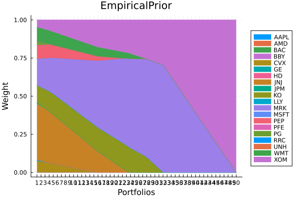
Empirical prior frontier.
r = StandardDeviation()
plot_measures(ress[1].w, prs[1]; x = r, y = ExpectedReturn(; rt = ress[1].ret),
              c = ExpectedReturnRiskRatio(; rt = ress[1].ret, rk = r, rf = 4.2 / 100 / 252),
              title = "EmpiricalPrior", xlabel = "SD", ylabel = "Arithmetic Return",
              colorbar_title = "\nRisk/Return Ratio", right_margin = 6Plots.mm)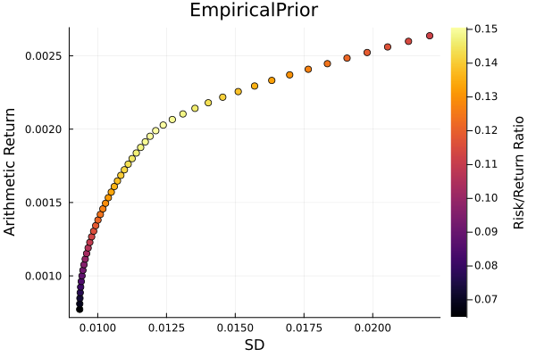
Factor prior composition with stepwise regression.
plot_stacked_area_composition(ress[2].w, rd.nx;
                              kwargs = (; xlabel = "Portfolios", ylabel = "Weight",
                                        title = "FactorPrior(Step)", legend = :outerright))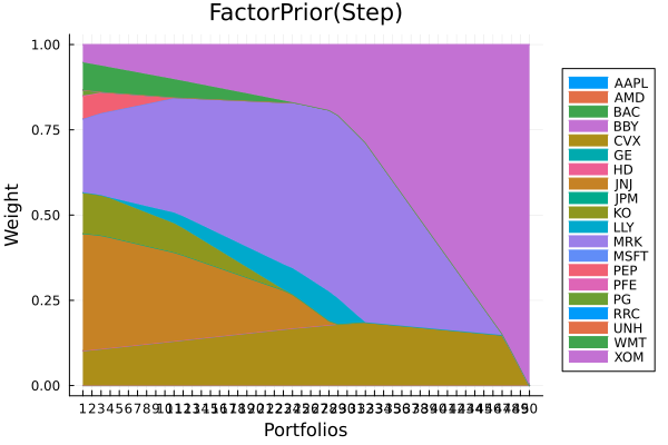
Factor prior frontier with stepwise regression.
r = StandardDeviation()
plot_measures(ress[2].w, prs[2]; x = r, y = ExpectedReturn(; rt = ress[2].ret),
              c = ExpectedReturnRiskRatio(; rt = ress[2].ret, rk = r, rf = 4.2 / 100 / 252),
              title = "FactorPrior(Step)", xlabel = "SD", ylabel = "Arithmetic Return",
              colorbar_title = "\nRisk/Return Ratio", right_margin = 6Plots.mm)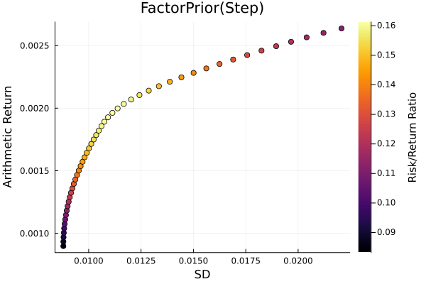
Factor prior using dimensionality reduction.
plot_stacked_area_composition(ress[3].w, rd.nx;
                              kwargs = (; xlabel = "Portfolios", ylabel = "Weight",
                                        title = "FactorPrior(DimRed)",
                                        legend = :outerright))
Factor prior frontier with stepwise regression.
r = StandardDeviation()
plot_measures(ress[3].w, prs[3]; x = r, y = ExpectedReturn(; rt = ress[3].ret),
              c = ExpectedReturnRiskRatio(; rt = ress[3].ret, rk = r, rf = 4.2 / 100 / 252),
              title = "FactorPrior(DimRed)", xlabel = "SD", ylabel = "Arithmetic Return",
              colorbar_title = "\nRisk/Return Ratio", right_margin = 6Plots.mm)
Let's optimise the maximum risk-adjusted return ratio of the three to see how a single portfolio differs.
opts = [JuMPOptimiser(; pe = prs[1], slv = slv), JuMPOptimiser(; pe = prs[2], slv = slv),
        JuMPOptimiser(; pe = prs[3], slv = slv)]

# Mean-Risk estimators using the standard deviation.
mrs = [MeanRisk(; r = StandardDeviation(), obj = MaximumRatio(; rf = 4.2 / 100 / 252),
                opt = opt) for opt in opts]

# Optimise
ress = optimise.(mrs)
pretty_table(DataFrame("Assets" => rd.nx, "EmpiricalPrior" => ress[1].w,
                       "FactorPrior(Step)" => ress[2].w,
                       "FactorPrior(DimRed)" => ress[3].w); formatters = [resfmt])
┌────────┬────────────────┬───────────────────┬─────────────────────┐
│ Assets │ EmpiricalPrior │ FactorPrior(Step) │ FactorPrior(DimRed) │
│ String │ Float64 │ Float64 │ Float64 │
├────────┼────────────────┼───────────────────┼─────────────────────┤
│ AAPL │ 0.0 % │ 0.0 % │ 0.0 % │
│ AMD │ 0.0 % │ 0.0 % │ 0.0 % │
│ BAC │ 0.0 % │ 0.0 % │ 0.0 % │
│ BBY │ 0.0 % │ 0.0 % │ 0.0 % │
│ CVX │ 0.0 % │ 18.328 % │ 16.403 % │
│ GE │ 0.0 % │ 0.0 % │ 0.0 % │
│ HD │ 0.0 % │ 0.0 % │ 0.0 % │
│ JNJ │ 0.0 % │ 0.0 % │ 0.0 % │
│ JPM │ 0.0 % │ 0.0 % │ 0.0 % │
│ KO │ 0.0 % │ 0.0 % │ 0.0 % │
│ LLY │ 0.0 % │ 3.133 % │ 4.507 % │
│ MRK │ 66.038 % │ 53.251 % │ 53.12 % │
│ MSFT │ 0.0 % │ 0.0 % │ 0.0 % │
│ PEP │ 0.0 % │ 0.0 % │ 0.0 % │
│ PFE │ 0.0 % │ 0.0 % │ 0.0 % │
│ ⋮ │ ⋮ │ ⋮ │ ⋮ │
└────────┴────────────────┴───────────────────┴─────────────────────┘
5 rows omittedWe can see that the factor model portfolios are more diversified than the empirical one. This is because the factor model reduces estimation error in the covariance matrix, leading to more stable and diversified portfolios.
3.2 Mean-NegativeSkewness optimisation
Here we will perform the exact same procedure as before, but using the negative skewness as the risk measure.
# JuMP Optimsiers, we will compute the efficient frontier with 50 points for all of them.
opts = [JuMPOptimiser(; pe = prs[4], slv = slv,
                      ret = ArithmeticReturn(; lb = Frontier(; N = 50))),
        JuMPOptimiser(; pe = prs[7], slv = slv,
                      ret = ArithmeticReturn(; lb = Frontier(; N = 50))),
        JuMPOptimiser(; pe = prs[8], slv = slv,
                      ret = ArithmeticReturn(; lb = Frontier(; N = 50)))]

# Mean-Risk estimators using the standard deviation.
mrs = [MeanRisk(; r = NegativeSkewness(), obj = MinimumRisk(), opt = opt) for opt in opts]

# Optimise
ress = optimise.(mrs)
3-element Vector{MeanRiskResult{DataType, __T_pa, Vector{OptimisationReturnCode}, Vector{JuMPOptimisationSolution}, Model, Nothing} where __T_pa}:
MeanRiskResult
oe ┼ DataType: DataType
pa ┼ ProcessedJuMPOptimiserAttributes
│ pr ┼ HighOrderPrior
│ │ pr ┼ LowOrderPrior
│ │ │ X ┼ 252×20 Matrix{Float64}
│ │ │ mu ┼ 20-element Vector{Float64}
│ │ │ sigma ┼ 20×20 Matrix{Float64}
│ │ │ chol ┼ nothing
│ │ │ w ┼ nothing
│ │ │ ens ┼ nothing
│ │ │ kld ┼ nothing
│ │ │ ow ┼ nothing
│ │ │ rr ┼ nothing
│ │ │ f_mu ┼ nothing
│ │ │ f_sigma ┼ nothing
│ │ │ f_w ┴ nothing
│ │ kt ┼ 400×400 Matrix{Float64}
│ │ L2 ┼ 210×400 SparseArrays.SparseMatrixCSC{Int64, Int64}
│ │ S2 ┼ 210×400 SparseArrays.SparseMatrixCSC{Int64, Int64}
│ │ sk ┼ 20×400 Matrix{Float64}
│ │ V ┼ 20×20 Matrix{Float64}
│ │ skmp ┼ DenoiseDetoneAlgMatrixProcessing
│ │ │ pdm ┼ Posdef
│ │ │ │ alg ┼ UnionAll: NearestCorrelationMatrix.Newton
│ │ │ │ kwargs ┴ @NamedTuple{}: NamedTuple()
│ │ │ dn ┼ nothing
│ │ │ dt ┼ nothing
│ │ │ alg ┼ nothing
│ │ │ order ┴ DenoiseDetoneAlg()
│ │ f_kt ┼ nothing
│ │ f_sk ┼ nothing
│ │ f_V ┴ nothing
│ wb ┼ WeightBounds
│ │ lb ┼ 20-element StepRangeLen{Float64, Base.TwicePrecision{Float64}, Base.TwicePrecision{Float64}, Int64}
│ │ ub ┴ 20-element StepRangeLen{Float64, Base.TwicePrecision{Float64}, Base.TwicePrecision{Float64}, Int64}
│ lt ┼ nothing
│ st ┼ nothing
│ lcsr ┼ nothing
│ ctr ┼ nothing
│ gcardr ┼ nothing
│ sgcardr ┼ nothing
│ smtx ┼ nothing
│ sgmtx ┼ nothing
│ slt ┼ nothing
│ sst ┼ nothing
│ sglt ┼ nothing
│ sgst ┼ nothing
│ tn ┼ nothing
│ fees ┼ nothing
│ plr ┼ nothing
│ ret ┼ ArithmeticReturn
│ │ ucs ┼ nothing
│ │ lb ┼ Frontier
│ │ │ N ┼ Int64: 50
│ │ │ factor ┼ Int64: 1
│ │ │ flag ┴ Bool: true
│ │ mu ┴ 20-element Vector{Float64}
retcode ┼ 50-element Vector{OptimisationReturnCode}
sol ┼ 50-element Vector{JuMPOptimisationSolution}
model ┼ A JuMP Model
│ ├ solver: Clarabel
│ ├ objective_sense: MIN_SENSE
│ │ └ objective_function_type: AffExpr
│ ├ num_variables: 22
│ ├ num_constraints: 6
│ │ ├ AffExpr in MOI.EqualTo{Float64}: 1
│ │ ├ AffExpr in MOI.GreaterThan{Float64}: 1
│ │ ├ Vector{AffExpr} in MOI.Nonnegatives: 1
│ │ ├ Vector{AffExpr} in MOI.Nonpositives: 1
│ │ ├ Vector{AffExpr} in MOI.SecondOrderCone: 1
│ │ └ VariableRef in MOI.Parameter{Float64}: 1
│ └ Names registered in the model
│ └ :GV, :bgt, :cnskew_soc_1, :k, :lw, :nskew_risk_1, :obj_expr, :ret, :ret_frontier, :ret_lb, :ret_lb_var, :risk, :risk_vec, :sc, :so, :w, :w_lb, :w_ub
fb ┴ nothing
MeanRiskResult
oe ┼ DataType: DataType
pa ┼ ProcessedJuMPOptimiserAttributes
│ pr ┼ HighOrderPrior
│ │ pr ┼ LowOrderPrior
│ │ │ X ┼ 252×20 Matrix{Float64}
│ │ │ mu ┼ 20-element Vector{Float64}
│ │ │ sigma ┼ 20×20 Matrix{Float64}
│ │ │ chol ┼ 25×20 LinearAlgebra.Transpose{Float64, Matrix{Float64}}
│ │ │ w ┼ nothing
│ │ │ ens ┼ nothing
│ │ │ kld ┼ nothing
│ │ │ ow ┼ nothing
│ │ │ rr ┼ Regression
│ │ │ │ M ┼ 20×5 SubArray{Float64, 2, Matrix{Float64}, Tuple{Base.Slice{Base.OneTo{Int64}}, UnitRange{Int64}}, true}
│ │ │ │ L ┼ 20×5 SubArray{Float64, 2, Matrix{Float64}, Tuple{Base.Slice{Base.OneTo{Int64}}, UnitRange{Int64}}, true}
│ │ │ │ b ┴ 20-element SubArray{Float64, 1, Matrix{Float64}, Tuple{Base.Slice{Base.OneTo{Int64}}, Int64}, true}
│ │ │ f_mu ┼ Vector{Float64}: [-0.0007221367902182355, -0.0008384535501032073, -0.0006253517821839465, -0.0003358529620217417, -0.000559091885073412]
│ │ │ f_sigma ┼ 5×5 Matrix{Float64}
│ │ │ f_w ┴ nothing
│ │ kt ┼ 400×400 Matrix{Float64}
│ │ L2 ┼ 210×400 SparseArrays.SparseMatrixCSC{Int64, Int64}
│ │ S2 ┼ 210×400 SparseArrays.SparseMatrixCSC{Int64, Int64}
│ │ sk ┼ 20×400 Matrix{Float64}
│ │ V ┼ 20×20 Matrix{Float64}
│ │ skmp ┼ DenoiseDetoneAlgMatrixProcessing
│ │ │ pdm ┼ Posdef
│ │ │ │ alg ┼ UnionAll: NearestCorrelationMatrix.Newton
│ │ │ │ kwargs ┴ @NamedTuple{}: NamedTuple()
│ │ │ dn ┼ nothing
│ │ │ dt ┼ nothing
│ │ │ alg ┼ nothing
│ │ │ order ┴ DenoiseDetoneAlg()
│ │ f_kt ┼ 25×25 Matrix{Float64}
│ │ f_sk ┼ 5×25 Matrix{Float64}
│ │ f_V ┴ 5×5 Matrix{Float64}
│ wb ┼ WeightBounds
│ │ lb ┼ 20-element StepRangeLen{Float64, Base.TwicePrecision{Float64}, Base.TwicePrecision{Float64}, Int64}
│ │ ub ┴ 20-element StepRangeLen{Float64, Base.TwicePrecision{Float64}, Base.TwicePrecision{Float64}, Int64}
│ lt ┼ nothing
│ st ┼ nothing
│ lcsr ┼ nothing
│ ctr ┼ nothing
│ gcardr ┼ nothing
│ sgcardr ┼ nothing
│ smtx ┼ nothing
│ sgmtx ┼ nothing
│ slt ┼ nothing
│ sst ┼ nothing
│ sglt ┼ nothing
│ sgst ┼ nothing
│ tn ┼ nothing
│ fees ┼ nothing
│ plr ┼ nothing
│ ret ┼ ArithmeticReturn
│ │ ucs ┼ nothing
│ │ lb ┼ Frontier
│ │ │ N ┼ Int64: 50
│ │ │ factor ┼ Int64: 1
│ │ │ flag ┴ Bool: true
│ │ mu ┴ 20-element Vector{Float64}
retcode ┼ 50-element Vector{OptimisationReturnCode}
sol ┼ 50-element Vector{JuMPOptimisationSolution}
model ┼ A JuMP Model
│ ├ solver: Clarabel
│ ├ objective_sense: MIN_SENSE
│ │ └ objective_function_type: AffExpr
│ ├ num_variables: 22
│ ├ num_constraints: 6
│ │ ├ AffExpr in MOI.EqualTo{Float64}: 1
│ │ ├ AffExpr in MOI.GreaterThan{Float64}: 1
│ │ ├ Vector{AffExpr} in MOI.Nonnegatives: 1
│ │ ├ Vector{AffExpr} in MOI.Nonpositives: 1
│ │ ├ Vector{AffExpr} in MOI.SecondOrderCone: 1
│ │ └ VariableRef in MOI.Parameter{Float64}: 1
│ └ Names registered in the model
│ └ :GV, :bgt, :cnskew_soc_1, :k, :lw, :nskew_risk_1, :obj_expr, :ret, :ret_frontier, :ret_lb, :ret_lb_var, :risk, :risk_vec, :sc, :so, :w, :w_lb, :w_ub
fb ┴ nothing
MeanRiskResult
oe ┼ DataType: DataType
pa ┼ ProcessedJuMPOptimiserAttributes
│ pr ┼ HighOrderPrior
│ │ pr ┼ LowOrderPrior
│ │ │ X ┼ 252×20 Matrix{Float64}
│ │ │ mu ┼ 20-element Vector{Float64}
│ │ │ sigma ┼ 20×20 Matrix{Float64}
│ │ │ chol ┼ 25×20 LinearAlgebra.Transpose{Float64, Matrix{Float64}}
│ │ │ w ┼ nothing
│ │ │ ens ┼ nothing
│ │ │ kld ┼ nothing
│ │ │ ow ┼ nothing
│ │ │ rr ┼ Regression
│ │ │ │ M ┼ 20×5 SubArray{Float64, 2, Matrix{Float64}, Tuple{Base.Slice{Base.OneTo{Int64}}, UnitRange{Int64}}, true}
│ │ │ │ L ┼ 20×4 LinearAlgebra.Transpose{Float64, Matrix{Float64}}
│ │ │ │ b ┴ 20-element SubArray{Float64, 1, Matrix{Float64}, Tuple{Base.Slice{Base.OneTo{Int64}}, Int64}, true}
│ │ │ f_mu ┼ Vector{Float64}: [-0.0007221367902182355, -0.0008384535501032073, -0.0006253517821839465, -0.0003358529620217417, -0.000559091885073412]
│ │ │ f_sigma ┼ 5×5 Matrix{Float64}
│ │ │ f_w ┴ nothing
│ │ kt ┼ 400×400 Matrix{Float64}
│ │ L2 ┼ 210×400 SparseArrays.SparseMatrixCSC{Int64, Int64}
│ │ S2 ┼ 210×400 SparseArrays.SparseMatrixCSC{Int64, Int64}
│ │ sk ┼ 20×400 Matrix{Float64}
│ │ V ┼ 20×20 Matrix{Float64}
│ │ skmp ┼ DenoiseDetoneAlgMatrixProcessing
│ │ │ pdm ┼ Posdef
│ │ │ │ alg ┼ UnionAll: NearestCorrelationMatrix.Newton
│ │ │ │ kwargs ┴ @NamedTuple{}: NamedTuple()
│ │ │ dn ┼ nothing
│ │ │ dt ┼ nothing
│ │ │ alg ┼ nothing
│ │ │ order ┴ DenoiseDetoneAlg()
│ │ f_kt ┼ 25×25 Matrix{Float64}
│ │ f_sk ┼ 5×25 Matrix{Float64}
│ │ f_V ┴ 5×5 Matrix{Float64}
│ wb ┼ WeightBounds
│ │ lb ┼ 20-element StepRangeLen{Float64, Base.TwicePrecision{Float64}, Base.TwicePrecision{Float64}, Int64}
│ │ ub ┴ 20-element StepRangeLen{Float64, Base.TwicePrecision{Float64}, Base.TwicePrecision{Float64}, Int64}
│ lt ┼ nothing
│ st ┼ nothing
│ lcsr ┼ nothing
│ ctr ┼ nothing
│ gcardr ┼ nothing
│ sgcardr ┼ nothing
│ smtx ┼ nothing
│ sgmtx ┼ nothing
│ slt ┼ nothing
│ sst ┼ nothing
│ sglt ┼ nothing
│ sgst ┼ nothing
│ tn ┼ nothing
│ fees ┼ nothing
│ plr ┼ nothing
│ ret ┼ ArithmeticReturn
│ │ ucs ┼ nothing
│ │ lb ┼ Frontier
│ │ │ N ┼ Int64: 50
│ │ │ factor ┼ Int64: 1
│ │ │ flag ┴ Bool: true
│ │ mu ┴ 20-element Vector{Float64}
retcode ┼ 50-element Vector{OptimisationReturnCode}
sol ┼ 50-element Vector{JuMPOptimisationSolution}
model ┼ A JuMP Model
│ ├ solver: Clarabel
│ ├ objective_sense: MIN_SENSE
│ │ └ objective_function_type: AffExpr
│ ├ num_variables: 22
│ ├ num_constraints: 6
│ │ ├ AffExpr in MOI.EqualTo{Float64}: 1
│ │ ├ AffExpr in MOI.GreaterThan{Float64}: 1
│ │ ├ Vector{AffExpr} in MOI.Nonnegatives: 1
│ │ ├ Vector{AffExpr} in MOI.Nonpositives: 1
│ │ ├ Vector{AffExpr} in MOI.SecondOrderCone: 1
│ │ └ VariableRef in MOI.Parameter{Float64}: 1
│ └ Names registered in the model
│ └ :GV, :bgt, :cnskew_soc_1, :k, :lw, :nskew_risk_1, :obj_expr, :ret, :ret_frontier, :ret_lb, :ret_lb_var, :risk, :risk_vec, :sc, :so, :w, :w_lb, :w_ub
fb ┴ nothingLet's plot the efficient frontiers.
Empirical prior composition.
plot_stacked_area_composition(ress[1].w, rd.nx;
                              kwargs = (; xlabel = "Portfolios", ylabel = "Weight",
                                        title = "EmpiricalPrior", legend = :outerright))
Empirical prior frontier.
r = NegativeSkewness()
plot_measures(ress[1].w, prs[4]; x = r, y = ExpectedReturn(; rt = ress[1].ret),
              c = ExpectedReturnRiskRatio(; rt = ress[1].ret, rk = r, rf = 4.2 / 100 / 252),
              title = "EmpiricalPrior", xlabel = "NegativeSkewness",
              ylabel = "Arithmetic Return", colorbar_title = "\nRisk/Return Ratio",
              right_margin = 6Plots.mm)
Factor prior composition with stepwise regression.
plot_stacked_area_composition(ress[2].w, rd.nx;
                              kwargs = (; xlabel = "Portfolios", ylabel = "Weight",
                                        title = "FactorPrior(Step)", legend = :outerright))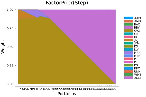
Factor prior frontier with stepwise regression.
r = NegativeSkewness()
plot_measures(ress[2].w, prs[7]; x = r, y = ExpectedReturn(; rt = ress[2].ret),
              c = ExpectedReturnRiskRatio(; rt = ress[2].ret, rk = r, rf = 4.2 / 100 / 252),
              title = "FactorPrior(Step)", xlabel = "NegativeSkewness",
              ylabel = "Arithmetic Return", colorbar_title = "\nRisk/Return Ratio",
              right_margin = 6Plots.mm)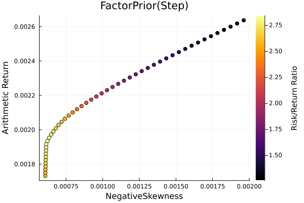
Factor prior using dimensionality reduction.
plot_stacked_area_composition(ress[3].w, rd.nx;
                              kwargs = (; xlabel = "Portfolios", ylabel = "Weight",
                                        title = "FactorPrior(DimRed)",
                                        legend = :outerright))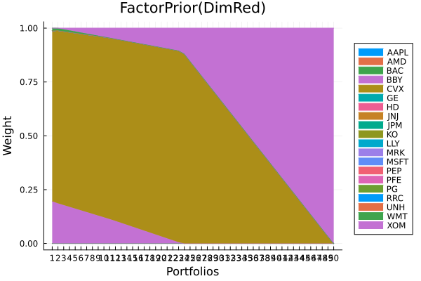
Factor prior frontier with stepwise regression.
r = NegativeSkewness()
plot_measures(ress[3].w, prs[8]; x = r, y = ExpectedReturn(; rt = ress[3].ret),
              c = ExpectedReturnRiskRatio(; rt = ress[3].ret, rk = r, rf = 4.2 / 100 / 252),
              title = "FactorPrior(DimRed)", xlabel = "NegativeSkewness",
              ylabel = "Arithmetic Return", colorbar_title = "\nRisk/Return Ratio",
              right_margin = 6Plots.mm)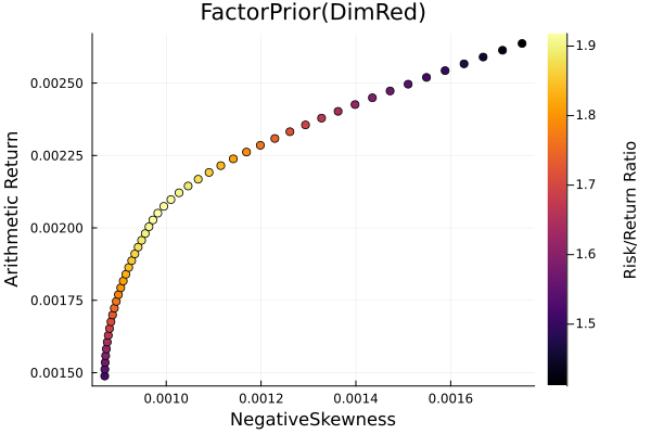
Let's optimise the maximum risk-adjusted return ratio of the three to see how a single portfolio differs.
opts = [JuMPOptimiser(; pe = prs[4], slv = slv), JuMPOptimiser(; pe = prs[7], slv = slv),
        JuMPOptimiser(; pe = prs[8], slv = slv)]

# Mean-Risk estimators using the standard deviation.
mrs = [MeanRisk(; r = NegativeSkewness(), obj = MaximumRatio(; rf = 4.2 / 100 / 252),
                opt = opt) for opt in opts]

# Optimise
ress = optimise.(mrs)
pretty_table(DataFrame("Assets" => rd.nx, "EmpiricalPrior" => ress[1].w,
                       "FactorPrior(Step)" => ress[2].w,
                       "FactorPrior(DimRed)" => ress[3].w); formatters = [resfmt])
┌────────┬────────────────┬───────────────────┬─────────────────────┐
│ Assets │ EmpiricalPrior │ FactorPrior(Step) │ FactorPrior(DimRed) │
│ String │ Float64 │ Float64 │ Float64 │
├────────┼────────────────┼───────────────────┼─────────────────────┤
│ AAPL │ 0.0 % │ 0.0 % │ 0.0 % │
│ AMD │ 0.0 % │ 0.0 % │ 0.0 % │
│ BAC │ 0.0 % │ 0.0 % │ 0.0 % │
│ BBY │ 0.0 % │ 0.0 % │ 0.0 % │
│ CVX │ 0.0 % │ 91.045 % │ 83.707 % │
│ GE │ 0.0 % │ 0.0 % │ 0.0 % │
│ HD │ 0.0 % │ 0.0 % │ 0.0 % │
│ JNJ │ 0.0 % │ 0.0 % │ 0.0 % │
│ JPM │ 0.0 % │ 0.0 % │ 0.0 % │
│ KO │ 0.0 % │ 0.0 % │ 0.0 % │
│ LLY │ 25.998 % │ 0.0 % │ 0.0 % │
│ MRK │ 58.385 % │ 8.955 % │ 0.0 % │
│ MSFT │ 0.0 % │ 0.0 % │ 0.0 % │
│ PEP │ 0.0 % │ 0.0 % │ 0.0 % │
│ PFE │ 0.0 % │ 0.0 % │ 0.0 % │
│ ⋮ │ ⋮ │ ⋮ │ ⋮ │
└────────┴────────────────┴───────────────────┴─────────────────────┘
5 rows omittedHere we have the opposite effect to before, this follows from the fact that for this particular scenario the condition number of the matrix of negative spectral slices of the coskewness is actually lower for the empirical prior than for the factor priors. This goes to show that higher order moments are more susceptible to noise, and factor models may not be able to fully mitigate this.
3.3 Mean-Kurtosis optimisation
Again we will do the same as before but with the kurtosis.
# JuMP Optimsiers, we will compute the efficient frontier with 50 points for all of them.
opts = [JuMPOptimiser(; pe = prs[4], slv = slv,
                      ret = ArithmeticReturn(; lb = Frontier(; N = 50))),
        JuMPOptimiser(; pe = prs[7], slv = slv,
                      ret = ArithmeticReturn(; lb = Frontier(; N = 50))),
        JuMPOptimiser(; pe = prs[8], slv = slv,
                      ret = ArithmeticReturn(; lb = Frontier(; N = 50)))]

# Mean-Risk estimators using the standard deviation.
mrs = [MeanRisk(; r = Kurtosis(), obj = MinimumRisk(), opt = opt) for opt in opts]

# Optimise
ress = optimise.(mrs)
3-element Vector{MeanRiskResult{DataType, __T_pa, Vector{OptimisationReturnCode}, Vector{JuMPOptimisationSolution}, Model, Nothing} where __T_pa}:
MeanRiskResult
oe ┼ DataType: DataType
pa ┼ ProcessedJuMPOptimiserAttributes
│ pr ┼ HighOrderPrior
│ │ pr ┼ LowOrderPrior
│ │ │ X ┼ 252×20 Matrix{Float64}
│ │ │ mu ┼ 20-element Vector{Float64}
│ │ │ sigma ┼ 20×20 Matrix{Float64}
│ │ │ chol ┼ nothing
│ │ │ w ┼ nothing
│ │ │ ens ┼ nothing
│ │ │ kld ┼ nothing
│ │ │ ow ┼ nothing
│ │ │ rr ┼ nothing
│ │ │ f_mu ┼ nothing
│ │ │ f_sigma ┼ nothing
│ │ │ f_w ┴ nothing
│ │ kt ┼ 400×400 Matrix{Float64}
│ │ L2 ┼ 210×400 SparseArrays.SparseMatrixCSC{Int64, Int64}
│ │ S2 ┼ 210×400 SparseArrays.SparseMatrixCSC{Int64, Int64}
│ │ sk ┼ 20×400 Matrix{Float64}
│ │ V ┼ 20×20 Matrix{Float64}
│ │ skmp ┼ DenoiseDetoneAlgMatrixProcessing
│ │ │ pdm ┼ Posdef
│ │ │ │ alg ┼ UnionAll: NearestCorrelationMatrix.Newton
│ │ │ │ kwargs ┴ @NamedTuple{}: NamedTuple()
│ │ │ dn ┼ nothing
│ │ │ dt ┼ nothing
│ │ │ alg ┼ nothing
│ │ │ order ┴ DenoiseDetoneAlg()
│ │ f_kt ┼ nothing
│ │ f_sk ┼ nothing
│ │ f_V ┴ nothing
│ wb ┼ WeightBounds
│ │ lb ┼ 20-element StepRangeLen{Float64, Base.TwicePrecision{Float64}, Base.TwicePrecision{Float64}, Int64}
│ │ ub ┴ 20-element StepRangeLen{Float64, Base.TwicePrecision{Float64}, Base.TwicePrecision{Float64}, Int64}
│ lt ┼ nothing
│ st ┼ nothing
│ lcsr ┼ nothing
│ ctr ┼ nothing
│ gcardr ┼ nothing
│ sgcardr ┼ nothing
│ smtx ┼ nothing
│ sgmtx ┼ nothing
│ slt ┼ nothing
│ sst ┼ nothing
│ sglt ┼ nothing
│ sgst ┼ nothing
│ tn ┼ nothing
│ fees ┼ nothing
│ plr ┼ nothing
│ ret ┼ ArithmeticReturn
│ │ ucs ┼ nothing
│ │ lb ┼ Frontier
│ │ │ N ┼ Int64: 50
│ │ │ factor ┼ Int64: 1
│ │ │ flag ┴ Bool: true
│ │ mu ┴ 20-element Vector{Float64}
retcode ┼ 50-element Vector{OptimisationReturnCode}
sol ┼ 50-element Vector{JuMPOptimisationSolution}
model ┼ A JuMP Model
│ ├ solver: Clarabel
│ ├ objective_sense: MIN_SENSE
│ │ └ objective_function_type: AffExpr
│ ├ num_variables: 232
│ ├ num_constraints: 7
│ │ ├ AffExpr in MOI.EqualTo{Float64}: 1
│ │ ├ AffExpr in MOI.GreaterThan{Float64}: 1
│ │ ├ Vector{AffExpr} in MOI.Nonnegatives: 1
│ │ ├ Vector{AffExpr} in MOI.Nonpositives: 1
│ │ ├ Vector{AffExpr} in MOI.SecondOrderCone: 1
│ │ ├ Vector{AffExpr} in MOI.PositiveSemidefiniteConeSquare: 1
│ │ └ VariableRef in MOI.Parameter{Float64}: 1
│ └ Names registered in the model
│ └ :Gkt, :L2W, :M, :M_PSD, :W, :bgt, :ckurt_soc_1, :k, :kurtosis_risk_1, :lw, :obj_expr, :ret, :ret_frontier, :ret_lb, :ret_lb_var, :risk, :risk_vec, :sc, :so, :w, :w_lb, :w_ub, :x_kurt_1
fb ┴ nothing
MeanRiskResult
oe ┼ DataType: DataType
pa ┼ ProcessedJuMPOptimiserAttributes
│ pr ┼ HighOrderPrior
│ │ pr ┼ LowOrderPrior
│ │ │ X ┼ 252×20 Matrix{Float64}
│ │ │ mu ┼ 20-element Vector{Float64}
│ │ │ sigma ┼ 20×20 Matrix{Float64}
│ │ │ chol ┼ 25×20 LinearAlgebra.Transpose{Float64, Matrix{Float64}}
│ │ │ w ┼ nothing
│ │ │ ens ┼ nothing
│ │ │ kld ┼ nothing
│ │ │ ow ┼ nothing
│ │ │ rr ┼ Regression
│ │ │ │ M ┼ 20×5 SubArray{Float64, 2, Matrix{Float64}, Tuple{Base.Slice{Base.OneTo{Int64}}, UnitRange{Int64}}, true}
│ │ │ │ L ┼ 20×5 SubArray{Float64, 2, Matrix{Float64}, Tuple{Base.Slice{Base.OneTo{Int64}}, UnitRange{Int64}}, true}
│ │ │ │ b ┴ 20-element SubArray{Float64, 1, Matrix{Float64}, Tuple{Base.Slice{Base.OneTo{Int64}}, Int64}, true}
│ │ │ f_mu ┼ Vector{Float64}: [-0.0007221367902182355, -0.0008384535501032073, -0.0006253517821839465, -0.0003358529620217417, -0.000559091885073412]
│ │ │ f_sigma ┼ 5×5 Matrix{Float64}
│ │ │ f_w ┴ nothing
│ │ kt ┼ 400×400 Matrix{Float64}
│ │ L2 ┼ 210×400 SparseArrays.SparseMatrixCSC{Int64, Int64}
│ │ S2 ┼ 210×400 SparseArrays.SparseMatrixCSC{Int64, Int64}
│ │ sk ┼ 20×400 Matrix{Float64}
│ │ V ┼ 20×20 Matrix{Float64}
│ │ skmp ┼ DenoiseDetoneAlgMatrixProcessing
│ │ │ pdm ┼ Posdef
│ │ │ │ alg ┼ UnionAll: NearestCorrelationMatrix.Newton
│ │ │ │ kwargs ┴ @NamedTuple{}: NamedTuple()
│ │ │ dn ┼ nothing
│ │ │ dt ┼ nothing
│ │ │ alg ┼ nothing
│ │ │ order ┴ DenoiseDetoneAlg()
│ │ f_kt ┼ 25×25 Matrix{Float64}
│ │ f_sk ┼ 5×25 Matrix{Float64}
│ │ f_V ┴ 5×5 Matrix{Float64}
│ wb ┼ WeightBounds
│ │ lb ┼ 20-element StepRangeLen{Float64, Base.TwicePrecision{Float64}, Base.TwicePrecision{Float64}, Int64}
│ │ ub ┴ 20-element StepRangeLen{Float64, Base.TwicePrecision{Float64}, Base.TwicePrecision{Float64}, Int64}
│ lt ┼ nothing
│ st ┼ nothing
│ lcsr ┼ nothing
│ ctr ┼ nothing
│ gcardr ┼ nothing
│ sgcardr ┼ nothing
│ smtx ┼ nothing
│ sgmtx ┼ nothing
│ slt ┼ nothing
│ sst ┼ nothing
│ sglt ┼ nothing
│ sgst ┼ nothing
│ tn ┼ nothing
│ fees ┼ nothing
│ plr ┼ nothing
│ ret ┼ ArithmeticReturn
│ │ ucs ┼ nothing
│ │ lb ┼ Frontier
│ │ │ N ┼ Int64: 50
│ │ │ factor ┼ Int64: 1
│ │ │ flag ┴ Bool: true
│ │ mu ┴ 20-element Vector{Float64}
retcode ┼ 50-element Vector{OptimisationReturnCode}
sol ┼ 50-element Vector{JuMPOptimisationSolution}
model ┼ A JuMP Model
│ ├ solver: Clarabel
│ ├ objective_sense: MIN_SENSE
│ │ └ objective_function_type: AffExpr
│ ├ num_variables: 232
│ ├ num_constraints: 7
│ │ ├ AffExpr in MOI.EqualTo{Float64}: 1
│ │ ├ AffExpr in MOI.GreaterThan{Float64}: 1
│ │ ├ Vector{AffExpr} in MOI.Nonnegatives: 1
│ │ ├ Vector{AffExpr} in MOI.Nonpositives: 1
│ │ ├ Vector{AffExpr} in MOI.SecondOrderCone: 1
│ │ ├ Vector{AffExpr} in MOI.PositiveSemidefiniteConeSquare: 1
│ │ └ VariableRef in MOI.Parameter{Float64}: 1
│ └ Names registered in the model
│ └ :Gkt, :L2W, :M, :M_PSD, :W, :bgt, :ckurt_soc_1, :k, :kurtosis_risk_1, :lw, :obj_expr, :ret, :ret_frontier, :ret_lb, :ret_lb_var, :risk, :risk_vec, :sc, :so, :w, :w_lb, :w_ub, :x_kurt_1
fb ┴ nothing
MeanRiskResult
oe ┼ DataType: DataType
pa ┼ ProcessedJuMPOptimiserAttributes
│ pr ┼ HighOrderPrior
│ │ pr ┼ LowOrderPrior
│ │ │ X ┼ 252×20 Matrix{Float64}
│ │ │ mu ┼ 20-element Vector{Float64}
│ │ │ sigma ┼ 20×20 Matrix{Float64}
│ │ │ chol ┼ 25×20 LinearAlgebra.Transpose{Float64, Matrix{Float64}}
│ │ │ w ┼ nothing
│ │ │ ens ┼ nothing
│ │ │ kld ┼ nothing
│ │ │ ow ┼ nothing
│ │ │ rr ┼ Regression
│ │ │ │ M ┼ 20×5 SubArray{Float64, 2, Matrix{Float64}, Tuple{Base.Slice{Base.OneTo{Int64}}, UnitRange{Int64}}, true}
│ │ │ │ L ┼ 20×4 LinearAlgebra.Transpose{Float64, Matrix{Float64}}
│ │ │ │ b ┴ 20-element SubArray{Float64, 1, Matrix{Float64}, Tuple{Base.Slice{Base.OneTo{Int64}}, Int64}, true}
│ │ │ f_mu ┼ Vector{Float64}: [-0.0007221367902182355, -0.0008384535501032073, -0.0006253517821839465, -0.0003358529620217417, -0.000559091885073412]
│ │ │ f_sigma ┼ 5×5 Matrix{Float64}
│ │ │ f_w ┴ nothing
│ │ kt ┼ 400×400 Matrix{Float64}
│ │ L2 ┼ 210×400 SparseArrays.SparseMatrixCSC{Int64, Int64}
│ │ S2 ┼ 210×400 SparseArrays.SparseMatrixCSC{Int64, Int64}
│ │ sk ┼ 20×400 Matrix{Float64}
│ │ V ┼ 20×20 Matrix{Float64}
│ │ skmp ┼ DenoiseDetoneAlgMatrixProcessing
│ │ │ pdm ┼ Posdef
│ │ │ │ alg ┼ UnionAll: NearestCorrelationMatrix.Newton
│ │ │ │ kwargs ┴ @NamedTuple{}: NamedTuple()
│ │ │ dn ┼ nothing
│ │ │ dt ┼ nothing
│ │ │ alg ┼ nothing
│ │ │ order ┴ DenoiseDetoneAlg()
│ │ f_kt ┼ 25×25 Matrix{Float64}
│ │ f_sk ┼ 5×25 Matrix{Float64}
│ │ f_V ┴ 5×5 Matrix{Float64}
│ wb ┼ WeightBounds
│ │ lb ┼ 20-element StepRangeLen{Float64, Base.TwicePrecision{Float64}, Base.TwicePrecision{Float64}, Int64}
│ │ ub ┴ 20-element StepRangeLen{Float64, Base.TwicePrecision{Float64}, Base.TwicePrecision{Float64}, Int64}
│ lt ┼ nothing
│ st ┼ nothing
│ lcsr ┼ nothing
│ ctr ┼ nothing
│ gcardr ┼ nothing
│ sgcardr ┼ nothing
│ smtx ┼ nothing
│ sgmtx ┼ nothing
│ slt ┼ nothing
│ sst ┼ nothing
│ sglt ┼ nothing
│ sgst ┼ nothing
│ tn ┼ nothing
│ fees ┼ nothing
│ plr ┼ nothing
│ ret ┼ ArithmeticReturn
│ │ ucs ┼ nothing
│ │ lb ┼ Frontier
│ │ │ N ┼ Int64: 50
│ │ │ factor ┼ Int64: 1
│ │ │ flag ┴ Bool: true
│ │ mu ┴ 20-element Vector{Float64}
retcode ┼ 50-element Vector{OptimisationReturnCode}
sol ┼ 50-element Vector{JuMPOptimisationSolution}
model ┼ A JuMP Model
│ ├ solver: Clarabel
│ ├ objective_sense: MIN_SENSE
│ │ └ objective_function_type: AffExpr
│ ├ num_variables: 232
│ ├ num_constraints: 7
│ │ ├ AffExpr in MOI.EqualTo{Float64}: 1
│ │ ├ AffExpr in MOI.GreaterThan{Float64}: 1
│ │ ├ Vector{AffExpr} in MOI.Nonnegatives: 1
│ │ ├ Vector{AffExpr} in MOI.Nonpositives: 1
│ │ ├ Vector{AffExpr} in MOI.SecondOrderCone: 1
│ │ ├ Vector{AffExpr} in MOI.PositiveSemidefiniteConeSquare: 1
│ │ └ VariableRef in MOI.Parameter{Float64}: 1
│ └ Names registered in the model
│ └ :Gkt, :L2W, :M, :M_PSD, :W, :bgt, :ckurt_soc_1, :k, :kurtosis_risk_1, :lw, :obj_expr, :ret, :ret_frontier, :ret_lb, :ret_lb_var, :risk, :risk_vec, :sc, :so, :w, :w_lb, :w_ub, :x_kurt_1
fb ┴ nothingLet's plot the efficient frontiers. However, this time when plotting the frontiers we will use the prior returns because the kurtosis risk measure is not computed from the cokurtosis matrix, but from the returns directly. Empirical prior composition.
plot_stacked_area_composition(ress[1].w, rd.nx;
                              kwargs = (; xlabel = "Portfolios", ylabel = "Weight",
                                        title = "EmpiricalPrior", legend = :outerright))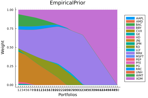
Empirical prior frontier.
r = Kurtosis()
plot_measures(ress[1].w, prs[4]; x = r, y = ExpectedReturn(; rt = ress[1].ret),
              c = ExpectedReturnRiskRatio(; rt = ress[1].ret, rk = r, rf = 4.2 / 100 / 252),
              title = "EmpiricalPrior", xlabel = "Kurtosis", ylabel = "Arithmetic Return",
              colorbar_title = "\nRisk/Return Ratio", right_margin = 6Plots.mm)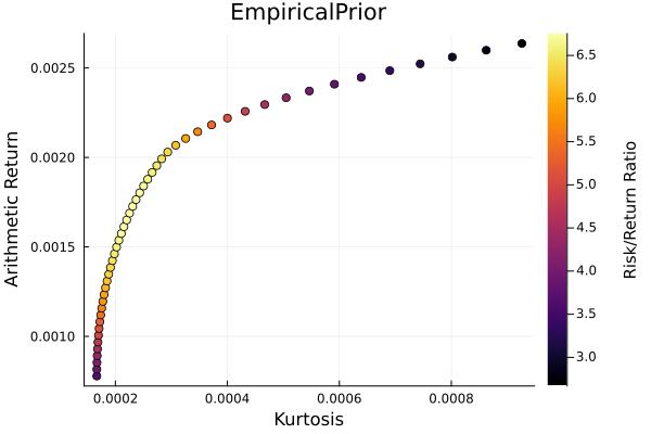
Factor prior composition with stepwise regression.
plot_stacked_area_composition(ress[2].w, rd.nx;
                              kwargs = (; xlabel = "Portfolios", ylabel = "Weight",
                                        title = "FactorPrior(Step)", legend = :outerright))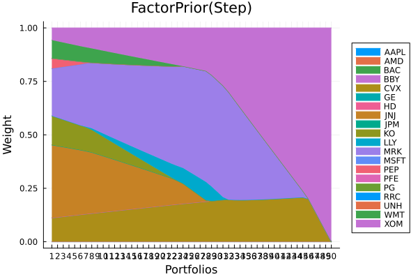
Factor prior frontier with stepwise regression.
r = Kurtosis()
plot_measures(ress[2].w, prs[4]; x = r, y = ExpectedReturn(; rt = ress[2].ret),
              c = ExpectedReturnRiskRatio(; rt = ress[2].ret, rk = r, rf = 4.2 / 100 / 252),
              title = "FactorPrior(Step)", xlabel = "Kurtosis",
              ylabel = "Arithmetic Return", colorbar_title = "\nRisk/Return Ratio",
              right_margin = 6Plots.mm)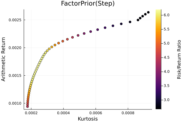
Factor prior using dimensionality reduction.
plot_stacked_area_composition(ress[3].w, rd.nx;
                              kwargs = (; xlabel = "Portfolios", ylabel = "Weight",
                                        title = "FactorPrior(DimRed)",
                                        legend = :outerright))
Factor prior frontier with stepwise regression.
r = Kurtosis()
plot_measures(ress[3].w, prs[4]; x = r, y = ExpectedReturn(; rt = ress[3].ret),
              c = ExpectedReturnRiskRatio(; rt = ress[3].ret, rk = r, rf = 4.2 / 100 / 252),
              title = "FactorPrior(DimRed)", xlabel = "Kurtosis",
              ylabel = "Arithmetic Return", colorbar_title = "\nRisk/Return Ratio",
              right_margin = 6Plots.mm)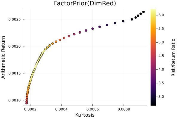
Let's optimise the maximum risk-adjusted return ratio of the three to see how a single portfolio differs.
opts = [JuMPOptimiser(; pe = prs[4], slv = slv), JuMPOptimiser(; pe = prs[7], slv = slv),
        JuMPOptimiser(; pe = prs[8], slv = slv)]

# Mean-Risk estimators using the standard deviation.
mrs = [MeanRisk(; r = NegativeSkewness(), obj = MaximumRatio(; rf = 4.2 / 100 / 252),
                opt = opt) for opt in opts]

# Optimise
ress = optimise.(mrs)
pretty_table(DataFrame("Assets" => rd.nx, "EmpiricalPrior" => ress[1].w,
                       "FactorPrior(Step)" => ress[2].w,
                       "FactorPrior(DimRed)" => ress[3].w); formatters = [resfmt])
┌────────┬────────────────┬───────────────────┬─────────────────────┐
│ Assets │ EmpiricalPrior │ FactorPrior(Step) │ FactorPrior(DimRed) │
│ String │ Float64 │ Float64 │ Float64 │
├────────┼────────────────┼───────────────────┼─────────────────────┤
│ AAPL │ 0.0 % │ 0.0 % │ 0.0 % │
│ AMD │ 0.0 % │ 0.0 % │ 0.0 % │
│ BAC │ 0.0 % │ 0.0 % │ 0.0 % │
│ BBY │ 0.0 % │ 0.0 % │ 0.0 % │
│ CVX │ 0.0 % │ 91.045 % │ 83.707 % │
│ GE │ 0.0 % │ 0.0 % │ 0.0 % │
│ HD │ 0.0 % │ 0.0 % │ 0.0 % │
│ JNJ │ 0.0 % │ 0.0 % │ 0.0 % │
│ JPM │ 0.0 % │ 0.0 % │ 0.0 % │
│ KO │ 0.0 % │ 0.0 % │ 0.0 % │
│ LLY │ 25.998 % │ 0.0 % │ 0.0 % │
│ MRK │ 58.385 % │ 8.955 % │ 0.0 % │
│ MSFT │ 0.0 % │ 0.0 % │ 0.0 % │
│ PEP │ 0.0 % │ 0.0 % │ 0.0 % │
│ PFE │ 0.0 % │ 0.0 % │ 0.0 % │
│ ⋮ │ ⋮ │ ⋮ │ ⋮ │
└────────┴────────────────┴───────────────────┴─────────────────────┘
5 rows omittedThese findings are again consistent with the previous result, and reflective of the higher condition numbers of the factor-based higher order statistics. The next example will explore ways of reducing the estimation error.
This page was generated using Literate.jl.