The source files for all examples can be found in /examples.

Example 9: Regularisation

This example shows one of the simplest ways to imporve the robustness of portfolios, regularisation penalties.

julia

using PortfolioOptimisers, PrettyTables
# Format for pretty tables.
tsfmt = (v, i, j) -> begin
    if j == 1
        return Date(v)
    else
        return v
    end
end;
resfmt = (v, i, j) -> begin
    if j == 1
        return v
    else
        return isa(v, Number) ? "$(round(v*100, digits=3)) %" : v
    end
end;
mmtfmt = (v, i, j) -> begin
    if i == j == 1
        return v
    else
        return isa(v, Number) ? "$(round(v*100, digits=3)) %" : v
    end
end;
summary_row = (data, j) -> begin
    if j == 1
        return "N/A"
    else
        return number_effective_assets(data[:, j])
    end
end

#11 (generic function with 1 method)

1. Setting up

We will use the same data as the previous example.

julia

using CSV, TimeSeries, DataFrames, Clarabel

X = TimeArray(CSV.File(joinpath(@__DIR__, "SP500.csv.gz")); timestamp = :Date)[(end - 252):end]
pretty_table(X[(end - 5):end]; formatters = [tsfmt])

# Compute the returns
rd = prices_to_returns(X)
pr = prior(EmpiricalPrior(), rd)

slv = [Solver(; name = :clarabel1, solver = Clarabel.Optimizer,
              settings = Dict("verbose" => false),
              check_sol = (; allow_local = true, allow_almost = true)),
       Solver(; name = :clarabel2, solver = Clarabel.Optimizer,
              settings = Dict("verbose" => false, "max_step_fraction" => 0.95),
              check_sol = (; allow_local = true, allow_almost = true)),
       Solver(; name = :clarabel3, solver = Clarabel.Optimizer,
              settings = Dict("verbose" => false, "max_step_fraction" => 0.9),
              check_sol = (; allow_local = true, allow_almost = true)),
       Solver(; name = :clarabel4, solver = Clarabel.Optimizer,
              settings = Dict("verbose" => false, "max_step_fraction" => 0.85),
              check_sol = (; allow_local = true, allow_almost = true)),
       Solver(; name = :clarabel5, solver = Clarabel.Optimizer,
              settings = Dict("verbose" => false, "max_step_fraction" => 0.8),
              check_sol = (; allow_local = true, allow_almost = true)),
       Solver(; name = :clarabel6, solver = Clarabel.Optimizer,
              settings = Dict("verbose" => false, "max_step_fraction" => 0.75),
              check_sol = (; allow_local = true, allow_almost = true)),
       Solver(; name = :clarabel7, solver = Clarabel.Optimizer,
              settings = Dict("verbose" => false, "max_step_fraction" => 0.70),
              check_sol = (; allow_local = true, allow_almost = true))];

┌────────────┬─────────┬─────────┬─────────┬─────────┬─────────┬─────────┬──────
│  timestamp │    AAPL │     AMD │     BAC │     BBY │     CVX │      GE │     ⋯
│ Dates.Date │ Float64 │ Float64 │ Float64 │ Float64 │ Float64 │ Float64 │ Flo ⋯
├────────────┼─────────┼─────────┼─────────┼─────────┼─────────┼─────────┼──────
│ 2022-12-20 │ 131.916 │   65.05 │  31.729 │  77.371 │ 169.497 │  62.604 │ 310 ⋯
│ 2022-12-21 │ 135.057 │   67.68 │  32.212 │  78.729 │  171.49 │   64.67 │ 314 ⋯
│ 2022-12-22 │ 131.846 │   63.86 │  31.927 │  78.563 │ 168.918 │  63.727 │ 311 ⋯
│ 2022-12-23 │ 131.477 │   64.52 │  32.005 │  79.432 │  174.14 │  63.742 │ 314 ⋯
│ 2022-12-27 │ 129.652 │   63.27 │  32.065 │   79.93 │ 176.329 │  64.561 │ 314 ⋯
│ 2022-12-28 │ 125.674 │   62.57 │  32.301 │  78.279 │ 173.728 │  63.883 │  31 ⋯
└────────────┴─────────┴─────────┴─────────┴─────────┴─────────┴─────────┴──────
                                                              14 columns omitted

2. Regularised portfolios

The optimal regularisation penalty value depends on the data, the investor preferences, and type of regularisation. The specific choice of penalty value is so volatile that it can only be estimated via cross-validation or similar techniques, but the "optimal" (to some definition of optimal) value will also change over time as the market conditions change. Therefore, we will simply show how to set up and solve a regularised portfolio optimisation problem, without attempting to find the optimal penalty value.

We will use the same small penalty for all regularisations to illustrate how they differ.

L1 regularisation (also known as Lasso regularisation) adds a penalty proportional to the sum of the absolute values of the portfolio weights. This encourages sparsity in the portfolio, leading to fewer assets being selected.
L2 regularisation (also known as Ridge regularisation) adds a penalty proportional to the sum of the squares of the portfolio weights. This discourages large weights and promotes diversification.
Lp regularisation via [LpRegularisation]-(@ref) adds a penalty proportional to the p-norm of the portfolio weights, where p > 1 is a positive real number.
L-Inf regularisation adds a penalty proportional to the maximum absolute value of the portfolio weights. This limits the influence of any single asset in the portfolio.

2.1 Efficient frontier

julia

opts = [JuMPOptimiser(; pr = pr, slv = slv, wb = WeightBounds(; lb = -1, ub = 1), sbgt = 1,
                      bgt = 1, ret = ArithmeticReturn(; lb = Frontier(; N = 50))),#
        JuMPOptimiser(; pr = pr, slv = slv, wb = WeightBounds(; lb = -1, ub = 1), sbgt = 1,
                      ret = ArithmeticReturn(; lb = Frontier(; N = 50)), bgt = 1,
                      l1 = 4e-4),#
        JuMPOptimiser(; pr = pr, slv = slv, wb = WeightBounds(; lb = -1, ub = 1), sbgt = 1,
                      ret = ArithmeticReturn(; lb = Frontier(; N = 50)), bgt = 1,
                      l2 = 4e-4),#
        JuMPOptimiser(; pr = pr, slv = slv, wb = WeightBounds(; lb = -1, ub = 1), sbgt = 1,
                      ret = ArithmeticReturn(; lb = Frontier(; N = 50)), bgt = 1,
                      lp = LpRegularisation(; p = 5, val = 4e-4)),#
        JuMPOptimiser(; pr = pr, slv = slv, wb = WeightBounds(; lb = -1, ub = 1), sbgt = 1,
                      ret = ArithmeticReturn(; lb = Frontier(; N = 50)), bgt = 1,
                      linf = 4e-4)]
nocs = [MeanRisk(; opt = opt) for opt in opts]
ress = optimise.(nocs)

5-element Vector{MeanRiskResult{DataType, ProcessedJuMPOptimiserAttributes{LowOrderPrior{Matrix{Float64}, Vector{Float64}, Matrix{Float64}, Nothing, Nothing, Nothing, Nothing, Nothing, Nothing, Nothing, Nothing, Nothing}, WeightBounds{StepRangeLen{Float64, Base.TwicePrecision{Float64}, Base.TwicePrecision{Float64}, Int64}, StepRangeLen{Float64, Base.TwicePrecision{Float64}, Base.TwicePrecision{Float64}, Int64}}, Nothing, Nothing, Nothing, Nothing, Nothing, Nothing, Nothing, Nothing, Nothing, Nothing, Nothing, Nothing, Nothing, Nothing, Nothing, ArithmeticReturn{Nothing, Frontier{Int64, Int64, Bool}, Nothing}}, Vector{OptimisationReturnCode}, Vector{JuMPOptimisationSolution}, JuMP.Model, Nothing}}:
 MeanRiskResult
       oe ┼ DataType: DataType
       pa ┼ ProcessedJuMPOptimiserAttributes
          │       pr ┼ LowOrderPrior
          │          │         X ┼ 252×20 Matrix{Float64}
          │          │        mu ┼ 20-element Vector{Float64}
          │          │     sigma ┼ 20×20 Matrix{Float64}
          │          │      chol ┼ nothing
          │          │         w ┼ nothing
          │          │       ens ┼ nothing
          │          │       kld ┼ nothing
          │          │        ow ┼ nothing
          │          │        rr ┼ nothing
          │          │      f_mu ┼ nothing
          │          │   f_sigma ┼ nothing
          │          │       f_w ┴ nothing
          │       wb ┼ WeightBounds
          │          │   lb ┼ 20-element StepRangeLen{Float64, Base.TwicePrecision{Float64}, Base.TwicePrecision{Float64}, Int64}
          │          │   ub ┴ 20-element StepRangeLen{Float64, Base.TwicePrecision{Float64}, Base.TwicePrecision{Float64}, Int64}
          │       lt ┼ nothing
          │       st ┼ nothing
          │      lcs ┼ nothing
          │       ct ┼ nothing
          │    gcard ┼ nothing
          │   sgcard ┼ nothing
          │     smtx ┼ nothing
          │    sgmtx ┼ nothing
          │      slt ┼ nothing
          │      sst ┼ nothing
          │     sglt ┼ nothing
          │     sgst ┼ nothing
          │       tn ┼ nothing
          │     fees ┼ nothing
          │       pl ┼ nothing
          │      ret ┼ ArithmeticReturn
          │          │   ucs ┼ nothing
          │          │    lb ┼ Frontier
          │          │       │        N ┼ Int64: 50
          │          │       │   factor ┼ Int64: 1
          │          │       │     flag ┴ Bool: true
          │          │    mu ┴ nothing
  retcode ┼ 50-element Vector{OptimisationReturnCode}
      sol ┼ 50-element Vector{JuMPOptimisationSolution}
    model ┼ A JuMP Model
          │ ├ solver: Clarabel
          │ ├ objective_sense: MIN_SENSE
          │ │ └ objective_function_type: JuMP.QuadExpr
          │ ├ num_variables: 61
          │ ├ num_constraints: 49
          │ │ ├ JuMP.AffExpr in MOI.EqualTo{Float64}: 3
          │ │ ├ JuMP.AffExpr in MOI.GreaterThan{Float64}: 1
          │ │ ├ Vector{JuMP.AffExpr} in MOI.Nonnegatives: 2
          │ │ ├ Vector{JuMP.AffExpr} in MOI.Nonpositives: 2
          │ │ ├ Vector{JuMP.AffExpr} in MOI.SecondOrderCone: 1
          │ │ └ JuMP.VariableRef in MOI.GreaterThan{Float64}: 40
          │ └ Names registered in the model
          │   └ :G, :bgt, :dev_1, :dev_1_soc, :k, :lbgt, :lw, :obj_expr, :ret, :ret_frontier, :ret_lb, :risk, :risk_vec, :sbgt, :sc, :so, :sw, :variance_flag, :variance_risk_1, :w, :w_lb, :w_lw, :w_sw, :w_ub
       fb ┴ nothing

 MeanRiskResult
       oe ┼ DataType: DataType
       pa ┼ ProcessedJuMPOptimiserAttributes
          │       pr ┼ LowOrderPrior
          │          │         X ┼ 252×20 Matrix{Float64}
          │          │        mu ┼ 20-element Vector{Float64}
          │          │     sigma ┼ 20×20 Matrix{Float64}
          │          │      chol ┼ nothing
          │          │         w ┼ nothing
          │          │       ens ┼ nothing
          │          │       kld ┼ nothing
          │          │        ow ┼ nothing
          │          │        rr ┼ nothing
          │          │      f_mu ┼ nothing
          │          │   f_sigma ┼ nothing
          │          │       f_w ┴ nothing
          │       wb ┼ WeightBounds
          │          │   lb ┼ 20-element StepRangeLen{Float64, Base.TwicePrecision{Float64}, Base.TwicePrecision{Float64}, Int64}
          │          │   ub ┴ 20-element StepRangeLen{Float64, Base.TwicePrecision{Float64}, Base.TwicePrecision{Float64}, Int64}
          │       lt ┼ nothing
          │       st ┼ nothing
          │      lcs ┼ nothing
          │       ct ┼ nothing
          │    gcard ┼ nothing
          │   sgcard ┼ nothing
          │     smtx ┼ nothing
          │    sgmtx ┼ nothing
          │      slt ┼ nothing
          │      sst ┼ nothing
          │     sglt ┼ nothing
          │     sgst ┼ nothing
          │       tn ┼ nothing
          │     fees ┼ nothing
          │       pl ┼ nothing
          │      ret ┼ ArithmeticReturn
          │          │   ucs ┼ nothing
          │          │    lb ┼ Frontier
          │          │       │        N ┼ Int64: 50
          │          │       │   factor ┼ Int64: 1
          │          │       │     flag ┴ Bool: true
          │          │    mu ┴ nothing
  retcode ┼ 50-element Vector{OptimisationReturnCode}
      sol ┼ 50-element Vector{JuMPOptimisationSolution}
    model ┼ A JuMP Model
          │ ├ solver: Clarabel
          │ ├ objective_sense: MIN_SENSE
          │ │ └ objective_function_type: JuMP.QuadExpr
          │ ├ num_variables: 62
          │ ├ num_constraints: 50
          │ │ ├ JuMP.AffExpr in MOI.EqualTo{Float64}: 3
          │ │ ├ JuMP.AffExpr in MOI.GreaterThan{Float64}: 1
          │ │ ├ Vector{JuMP.AffExpr} in MOI.Nonnegatives: 2
          │ │ ├ Vector{JuMP.AffExpr} in MOI.Nonpositives: 2
          │ │ ├ Vector{JuMP.AffExpr} in MOI.NormOneCone: 1
          │ │ ├ Vector{JuMP.AffExpr} in MOI.SecondOrderCone: 1
          │ │ └ JuMP.VariableRef in MOI.GreaterThan{Float64}: 40
          │ └ Names registered in the model
          │   └ :G, :bgt, :cl1_noc, :dev_1, :dev_1_soc, :k, :l1, :lbgt, :lw, :obj_expr, :op, :ret, :ret_frontier, :ret_lb, :risk, :risk_vec, :sbgt, :sc, :so, :sw, :t_l1, :variance_flag, :variance_risk_1, :w, :w_lb, :w_lw, :w_sw, :w_ub
       fb ┴ nothing

 MeanRiskResult
       oe ┼ DataType: DataType
       pa ┼ ProcessedJuMPOptimiserAttributes
          │       pr ┼ LowOrderPrior
          │          │         X ┼ 252×20 Matrix{Float64}
          │          │        mu ┼ 20-element Vector{Float64}
          │          │     sigma ┼ 20×20 Matrix{Float64}
          │          │      chol ┼ nothing
          │          │         w ┼ nothing
          │          │       ens ┼ nothing
          │          │       kld ┼ nothing
          │          │        ow ┼ nothing
          │          │        rr ┼ nothing
          │          │      f_mu ┼ nothing
          │          │   f_sigma ┼ nothing
          │          │       f_w ┴ nothing
          │       wb ┼ WeightBounds
          │          │   lb ┼ 20-element StepRangeLen{Float64, Base.TwicePrecision{Float64}, Base.TwicePrecision{Float64}, Int64}
          │          │   ub ┴ 20-element StepRangeLen{Float64, Base.TwicePrecision{Float64}, Base.TwicePrecision{Float64}, Int64}
          │       lt ┼ nothing
          │       st ┼ nothing
          │      lcs ┼ nothing
          │       ct ┼ nothing
          │    gcard ┼ nothing
          │   sgcard ┼ nothing
          │     smtx ┼ nothing
          │    sgmtx ┼ nothing
          │      slt ┼ nothing
          │      sst ┼ nothing
          │     sglt ┼ nothing
          │     sgst ┼ nothing
          │       tn ┼ nothing
          │     fees ┼ nothing
          │       pl ┼ nothing
          │      ret ┼ ArithmeticReturn
          │          │   ucs ┼ nothing
          │          │    lb ┼ Frontier
          │          │       │        N ┼ Int64: 50
          │          │       │   factor ┼ Int64: 1
          │          │       │     flag ┴ Bool: true
          │          │    mu ┴ nothing
  retcode ┼ 50-element Vector{OptimisationReturnCode}
      sol ┼ 50-element Vector{JuMPOptimisationSolution}
    model ┼ A JuMP Model
          │ ├ solver: Clarabel
          │ ├ objective_sense: MIN_SENSE
          │ │ └ objective_function_type: JuMP.QuadExpr
          │ ├ num_variables: 62
          │ ├ num_constraints: 50
          │ │ ├ JuMP.AffExpr in MOI.EqualTo{Float64}: 3
          │ │ ├ JuMP.AffExpr in MOI.GreaterThan{Float64}: 1
          │ │ ├ Vector{JuMP.AffExpr} in MOI.Nonnegatives: 2
          │ │ ├ Vector{JuMP.AffExpr} in MOI.Nonpositives: 2
          │ │ ├ Vector{JuMP.AffExpr} in MOI.SecondOrderCone: 2
          │ │ └ JuMP.VariableRef in MOI.GreaterThan{Float64}: 40
          │ └ Names registered in the model
          │   └ :G, :bgt, :cl2_soc, :dev_1, :dev_1_soc, :k, :l2, :lbgt, :lw, :obj_expr, :op, :ret, :ret_frontier, :ret_lb, :risk, :risk_vec, :sbgt, :sc, :so, :sw, :t_l2, :variance_flag, :variance_risk_1, :w, :w_lb, :w_lw, :w_sw, :w_ub
       fb ┴ nothing

 MeanRiskResult
       oe ┼ DataType: DataType
       pa ┼ ProcessedJuMPOptimiserAttributes
          │       pr ┼ LowOrderPrior
          │          │         X ┼ 252×20 Matrix{Float64}
          │          │        mu ┼ 20-element Vector{Float64}
          │          │     sigma ┼ 20×20 Matrix{Float64}
          │          │      chol ┼ nothing
          │          │         w ┼ nothing
          │          │       ens ┼ nothing
          │          │       kld ┼ nothing
          │          │        ow ┼ nothing
          │          │        rr ┼ nothing
          │          │      f_mu ┼ nothing
          │          │   f_sigma ┼ nothing
          │          │       f_w ┴ nothing
          │       wb ┼ WeightBounds
          │          │   lb ┼ 20-element StepRangeLen{Float64, Base.TwicePrecision{Float64}, Base.TwicePrecision{Float64}, Int64}
          │          │   ub ┴ 20-element StepRangeLen{Float64, Base.TwicePrecision{Float64}, Base.TwicePrecision{Float64}, Int64}
          │       lt ┼ nothing
          │       st ┼ nothing
          │      lcs ┼ nothing
          │       ct ┼ nothing
          │    gcard ┼ nothing
          │   sgcard ┼ nothing
          │     smtx ┼ nothing
          │    sgmtx ┼ nothing
          │      slt ┼ nothing
          │      sst ┼ nothing
          │     sglt ┼ nothing
          │     sgst ┼ nothing
          │       tn ┼ nothing
          │     fees ┼ nothing
          │       pl ┼ nothing
          │      ret ┼ ArithmeticReturn
          │          │   ucs ┼ nothing
          │          │    lb ┼ Frontier
          │          │       │        N ┼ Int64: 50
          │          │       │   factor ┼ Int64: 1
          │          │       │     flag ┴ Bool: true
          │          │    mu ┴ nothing
  retcode ┼ 50-element Vector{OptimisationReturnCode}
      sol ┼ 50-element Vector{JuMPOptimisationSolution}
    model ┼ A JuMP Model
          │ ├ solver: Clarabel
          │ ├ objective_sense: MIN_SENSE
          │ │ └ objective_function_type: JuMP.QuadExpr
          │ ├ num_variables: 82
          │ ├ num_constraints: 70
          │ │ ├ JuMP.AffExpr in MOI.EqualTo{Float64}: 4
          │ │ ├ JuMP.AffExpr in MOI.GreaterThan{Float64}: 1
          │ │ ├ Vector{JuMP.AffExpr} in MOI.Nonnegatives: 2
          │ │ ├ Vector{JuMP.AffExpr} in MOI.Nonpositives: 2
          │ │ ├ Vector{JuMP.AffExpr} in MOI.SecondOrderCone: 1
          │ │ ├ Vector{JuMP.AffExpr} in MOI.PowerCone{Float64}: 20
          │ │ └ JuMP.VariableRef in MOI.GreaterThan{Float64}: 40
          │ └ Names registered in the model
          │   └ :G, :bgt, :clp_1, :cslp_1, :dev_1, :dev_1_soc, :k, :lbgt, :lp_1, :lw, :obj_expr, :op, :r_lp_1, :ret, :ret_frontier, :ret_lb, :risk, :risk_vec, :sbgt, :sc, :so, :sw, :t_lp_1, :variance_flag, :variance_risk_1, :w, :w_lb, :w_lw, :w_sw, :w_ub
       fb ┴ nothing

 MeanRiskResult
       oe ┼ DataType: DataType
       pa ┼ ProcessedJuMPOptimiserAttributes
          │       pr ┼ LowOrderPrior
          │          │         X ┼ 252×20 Matrix{Float64}
          │          │        mu ┼ 20-element Vector{Float64}
          │          │     sigma ┼ 20×20 Matrix{Float64}
          │          │      chol ┼ nothing
          │          │         w ┼ nothing
          │          │       ens ┼ nothing
          │          │       kld ┼ nothing
          │          │        ow ┼ nothing
          │          │        rr ┼ nothing
          │          │      f_mu ┼ nothing
          │          │   f_sigma ┼ nothing
          │          │       f_w ┴ nothing
          │       wb ┼ WeightBounds
          │          │   lb ┼ 20-element StepRangeLen{Float64, Base.TwicePrecision{Float64}, Base.TwicePrecision{Float64}, Int64}
          │          │   ub ┴ 20-element StepRangeLen{Float64, Base.TwicePrecision{Float64}, Base.TwicePrecision{Float64}, Int64}
          │       lt ┼ nothing
          │       st ┼ nothing
          │      lcs ┼ nothing
          │       ct ┼ nothing
          │    gcard ┼ nothing
          │   sgcard ┼ nothing
          │     smtx ┼ nothing
          │    sgmtx ┼ nothing
          │      slt ┼ nothing
          │      sst ┼ nothing
          │     sglt ┼ nothing
          │     sgst ┼ nothing
          │       tn ┼ nothing
          │     fees ┼ nothing
          │       pl ┼ nothing
          │      ret ┼ ArithmeticReturn
          │          │   ucs ┼ nothing
          │          │    lb ┼ Frontier
          │          │       │        N ┼ Int64: 50
          │          │       │   factor ┼ Int64: 1
          │          │       │     flag ┴ Bool: true
          │          │    mu ┴ nothing
  retcode ┼ 50-element Vector{OptimisationReturnCode}
      sol ┼ 50-element Vector{JuMPOptimisationSolution}
    model ┼ A JuMP Model
          │ ├ solver: Clarabel
          │ ├ objective_sense: MIN_SENSE
          │ │ └ objective_function_type: JuMP.QuadExpr
          │ ├ num_variables: 62
          │ ├ num_constraints: 50
          │ │ ├ JuMP.AffExpr in MOI.EqualTo{Float64}: 3
          │ │ ├ JuMP.AffExpr in MOI.GreaterThan{Float64}: 1
          │ │ ├ Vector{JuMP.AffExpr} in MOI.Nonnegatives: 2
          │ │ ├ Vector{JuMP.AffExpr} in MOI.Nonpositives: 2
          │ │ ├ Vector{JuMP.AffExpr} in MOI.NormInfinityCone: 1
          │ │ ├ Vector{JuMP.AffExpr} in MOI.SecondOrderCone: 1
          │ │ └ JuMP.VariableRef in MOI.GreaterThan{Float64}: 40
          │ └ Names registered in the model
          │   └ :G, :bgt, :clinf_nic, :dev_1, :dev_1_soc, :k, :lbgt, :linf, :lw, :obj_expr, :op, :ret, :ret_frontier, :ret_lb, :risk, :risk_vec, :sbgt, :sc, :so, :sw, :t_linf, :variance_flag, :variance_risk_1, :w, :w_lb, :w_lw, :w_sw, :w_ub
       fb ┴ nothing

Let's plot the efficient frontiers.

julia

using GraphRecipes, StatsPlots

r = Variance()

Variance
  settings ┼ RiskMeasureSettings
           │   scale ┼ Float64: 1.0
           │      ub ┼ nothing
           │     rke ┴ Bool: true
     sigma ┼ nothing
      chol ┼ nothing
        rc ┼ nothing
       alg ┴ SquaredSOCRiskExpr()

No regularisation portfolio weights.

julia

plot_stacked_area_composition(ress[1].w, rd.nx;
                              kwargs = (; xlabel = "Portfolios", ylabel = "Weight",
                                        title = "No regularisation", legend = :outerright))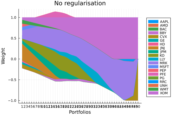

No regularisation frontier.

julia

plot_measures(ress[1].w, pr; x = r, y = ReturnRiskMeasure(; rt = ress[1].ret),
              c = ReturnRiskRatioRiskMeasure(; rt = ress[1].ret, rk = r,
                                             rf = 4.2 / 100 / 252),
              title = "No regularisation", xlabel = "Variance",
              ylabel = "Arithmetic Return", colorbar_title = "\nRisk/Return Ratio",
              right_margin = 6Plots.mm)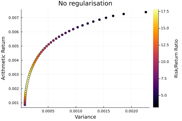

L1 regularisation portfolio weights. As expected, the portfolio is sparsified, with fewer assets with non-zero weight.

julia

plot_stacked_area_composition(ress[2].w, rd.nx;
                              kwargs = (; xlabel = "Portfolios", ylabel = "Weight",
                                        title = "L1 regularisation", legend = :outerright))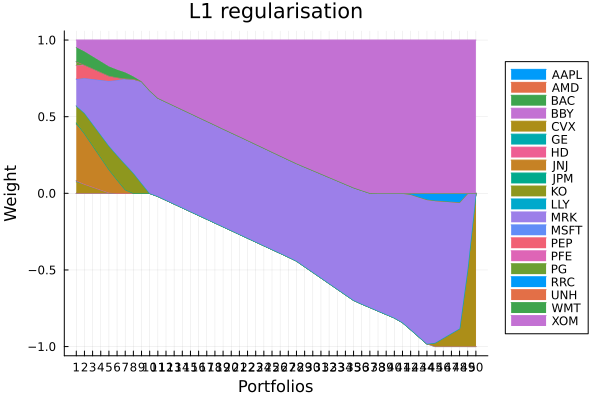

L1 regularisation frontier. The sparsification makes the pareto front non-smooth.

julia

plot_measures(ress[2].w, pr; x = r, y = ReturnRiskMeasure(; rt = ress[2].ret),
              c = ReturnRiskRatioRiskMeasure(; rt = ress[1].ret, rk = r,
                                             rf = 4.2 / 100 / 252),
              title = "L1 regularisation", xlabel = "Variance",
              ylabel = "Arithmetic Return", colorbar_title = "\nRisk/Return Ratio",
              right_margin = 6Plots.mm)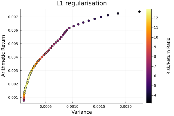

L2 regularisation portfolio weights. Even values of p-norms smooth out the weights, leading to more diversified portfolios. The higher the value, the more highly penalised larger deviations from the mean weight become. This is similar to how moments of even order behave.

julia

plot_stacked_area_composition(ress[3].w, rd.nx;
                              kwargs = (; xlabel = "Portfolios", ylabel = "Weight",
                                        title = "L2 regularisation", legend = :outerright))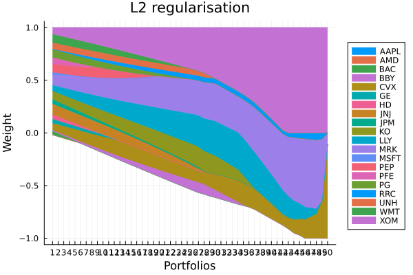

L2 regularisation frontier.

julia

plot_measures(ress[3].w, pr; x = r, y = ReturnRiskMeasure(; rt = ress[3].ret),
              c = ReturnRiskRatioRiskMeasure(; rt = ress[1].ret, rk = r,
                                             rf = 4.2 / 100 / 252),
              title = "L2 regularisation", xlabel = "Variance",
              ylabel = "Arithmetic Return", colorbar_title = "\nRisk/Return Ratio",
              right_margin = 6Plots.mm)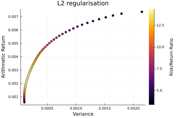

Lp regularisation portfolio weights. The higher the value of p, the closer the behaviour is to L-Inf regularisation, where the maximum absolute weight is penalised. This leads to portfolios where all weights are more similar in magnitude, but does not smear the negative weights into positive values like the L2 norm.

julia

plot_stacked_area_composition(ress[4].w, rd.nx;
                              kwargs = (; xlabel = "Portfolios", ylabel = "Weight",
                                        title = "Lp (p = 5) regularisation",
                                        legend = :outerright))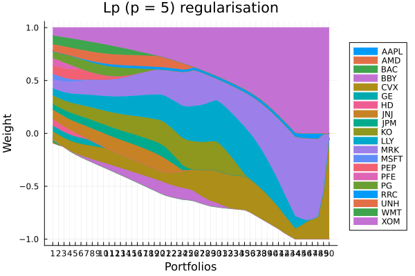

Lp regularisation frontier.

julia

plot_measures(ress[4].w, pr; x = r, y = ReturnRiskMeasure(; rt = ress[4].ret),
              c = ReturnRiskRatioRiskMeasure(; rt = ress[1].ret, rk = r,
                                             rf = 4.2 / 100 / 252),
              title = "Lp (p = 5) regularisation", xlabel = "Variance",
              ylabel = "Arithmetic Return", colorbar_title = "\nRisk/Return Ratio",
              right_margin = 6Plots.mm)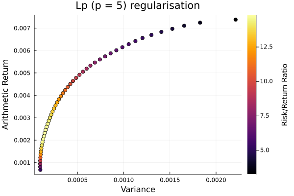

L-Inf regularisation portfolio weights.

julia

plot_stacked_area_composition(ress[5].w, rd.nx;
                              kwargs = (; xlabel = "Portfolios", ylabel = "Weight",
                                        title = "L-Inf regularisation",
                                        legend = :outerright))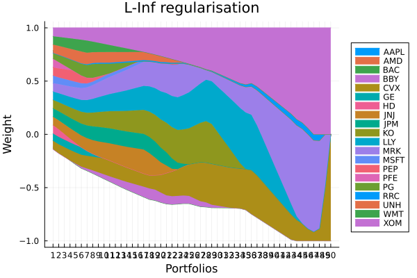

L-Inf regularisation frontier.

julia

plot_measures(ress[5].w, pr; x = r, y = ReturnRiskMeasure(; rt = ress[5].ret),
              c = ReturnRiskRatioRiskMeasure(; rt = ress[1].ret, rk = r,
                                             rf = 4.2 / 100 / 252),
              title = "L-Inf regularisation", xlabel = "Variance",
              ylabel = "Arithmetic Return", colorbar_title = "\nRisk/Return Ratio",
              right_margin = 6Plots.mm)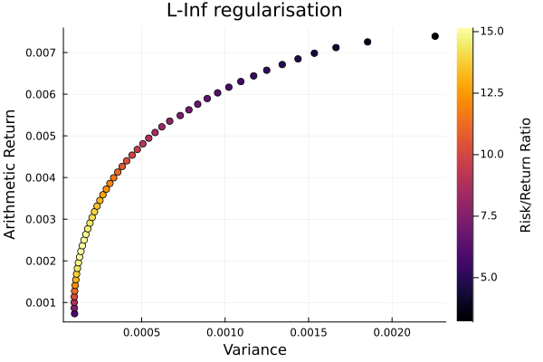

2.2 Minimum risk portfolios

Lets view only the minimum risk portfolios for each regularisation to get more insight into what regularisation does.

julia

opts = [JuMPOptimiser(; pr = pr, slv = slv, wb = WeightBounds(; lb = -1, ub = 1), sbgt = 1,
                      bgt = 1),# no regularisation
        JuMPOptimiser(; pr = pr, slv = slv, wb = WeightBounds(; lb = -1, ub = 1), sbgt = 1,
                      bgt = 1, l1 = 4e-4),# L1 regularisation
        JuMPOptimiser(; pr = pr, slv = slv, wb = WeightBounds(; lb = -1, ub = 1), sbgt = 1,
                      bgt = 1, l2 = 4e-4),# L2 regularisation
        JuMPOptimiser(; pr = pr, slv = slv, wb = WeightBounds(; lb = -1, ub = 1), sbgt = 1,
                      bgt = 1, lp = LpRegularisation(; p = 5, val = 4e-4)),# Lp regularisation with p = 5
        JuMPOptimiser(; pr = pr, slv = slv, wb = WeightBounds(; lb = -1, ub = 1), sbgt = 1,
                      bgt = 1, linf = 4e-4)]# L-Inf regularisation
nocs = [MeanRisk(; opt = opt) for opt in opts]

ress = optimise.(nocs)
pretty_table(DataFrame(:Assets => rd.nx, :No_Reg => ress[1].w, :L1 => ress[2].w,
                       :L2 => ress[3].w, :L5 => ress[4].w, :LInf => ress[5].w);
             formatters = [resfmt], summary_rows = [summary_row],
             summary_row_labels = ["# Eff. Assets"])

┌───────────────┬────────┬───────────┬──────────┬──────────┬──────────┬─────────
│               │ Assets │    No_Reg │       L1 │       L2 │       L5 │     LI ⋯
│               │ String │   Float64 │  Float64 │  Float64 │  Float64 │  Float ⋯
├───────────────┼────────┼───────────┼──────────┼──────────┼──────────┼─────────
│               │   AAPL │ -11.866 % │    0.0 % │  1.136 % │ -3.026 % │ -5.751 ⋯
│               │    AMD │   -1.55 % │    0.0 % │ -2.963 % │ -6.029 % │ -7.437 ⋯
│               │    BAC │   -5.46 % │    0.0 % │  3.488 % │   4.28 % │  1.181 ⋯
│               │    BBY │  -3.234 % │    0.0 % │  1.035 % │ -1.015 % │ -1.935 ⋯
│               │    CVX │   9.487 % │  7.415 % │   6.57 % │  7.553 % │  7.879 ⋯
│               │     GE │   5.203 % │  0.823 % │  3.871 % │  5.501 % │  6.838 ⋯
│               │     HD │   3.621 % │    0.0 % │  4.194 % │  6.143 % │  7.879 ⋯
│               │    JNJ │  40.958 % │ 36.981 % │ 10.221 % │   9.02 % │  7.879 ⋯
│               │    JPM │   7.738 % │  0.762 % │  4.252 % │  5.446 % │  7.879 ⋯
│               │     KO │    12.0 % │ 11.098 % │  7.952 % │  8.217 % │  7.879 ⋯
│               │    LLY │  -7.707 % │    0.0 % │  5.655 % │  6.507 % │  7.878 ⋯
│               │    MRK │  19.792 % │ 17.462 % │  9.638 % │  8.719 % │  7.879 ⋯
│               │   MSFT │   8.105 % │    0.0 % │  2.536 % │  4.917 % │  7.071 ⋯
│             ⋮ │      ⋮ │         ⋮ │        ⋮ │        ⋮ │        ⋮ │        ⋱
├───────────────┼────────┼───────────┼──────────┼──────────┼──────────┼─────────
│ # Eff. Assets │    N/A │   3.28601 │  4.88263 │  13.8946 │   11.588 │    9.9 ⋯
└───────────────┴────────┴───────────┴──────────┴──────────┴──────────┴─────────
                                                     1 column and 7 rows omitted

The effect of each regularisation depends on the relative values of the objective function with respect to the value of the relevant norm of the optimised portfolio weights multiplied by the penalty.

Generally, regularised portfolios tend to have more effective assets than unregularised ones. The number of effective assets is different to the sparsity in that it measures the concentration of weights as 1/(w ⋅ w), rather than counting the number of non-zero (or near zero) weights. Usually, the larger the number of effective assets, the more diversified the portfolio. Sparsity is a non-smooth measure, while the number of effective assets is smooth, so a portfolio can have higher sparsity and still have a larger number of effective assets.

It is possible to combine multiple regularisation penalties in the same optimisation problem by simultaneously specifying multiple regularisation keywords in the JuMPOptimiser. This can be useful to combine the benefits of different regularisations, such as sparsity and diversification, but can make the optimisation more difficult to solve and interpret.

This page was generated using Literate.jl.

Constraints

Risk Constraints

Example 9: Regularisation

1. Setting up

2. Regularised portfolios

2.1 Efficient frontier

2.2 Minimum risk portfolios

Example 9: Regularisation ​

1. Setting up ​

2. Regularised portfolios ​

2.1 Efficient frontier ​

2.2 Minimum risk portfolios ​

Example 9: Regularisation

1. Setting up

2. Regularised portfolios

2.1 Efficient frontier

2.2 Minimum risk portfolios