The source files can be found in examples/.
Example 3: Efficient frontier
In this example we will show how to compute efficient frontiers using the MeanRisk and NearOptimalCentering estimators.
using PortfolioOptimisers, PrettyTables
# Format for pretty tables.
tsfmt = (v, i, j) -> begin
    if j == 1
        return Date(v)
    else
        return v
    end
end;
resfmt = (v, i, j) -> begin
    if j == 1
        return v
    else
        return isa(v, Number) ? "$(round(v*100, digits=3)) %" : v
    end
end;
1. ReturnsResult data
We will use the same data as the previous example.
using CSV, TimeSeries, DataFrames

X = TimeArray(CSV.File(joinpath(@__DIR__, "SP500.csv.gz")); timestamp = :Date)[(end - 252):end]
pretty_table(X[(end - 5):end]; formatters = [tsfmt])

# Compute the returns
rd = prices_to_returns(X)
ReturnsResult
nx ┼ 20-element Vector{String}
X ┼ 252×20 Matrix{Float64}
nf ┼ nothing
F ┼ nothing
nb ┼ nothing
B ┼ nothing
ts ┼ 252-element Vector{Date}
iv ┼ nothing
ivpa ┴ nothing2. Efficient frontier
We have two mutually exclusive ways to compute the efficient frontier. We can do so from the perspective of minimising the risk with a return lower bound, or maximising the return with a risk upper bound. It is possible to provide explicit bounds, or a Frontier object which automatically computes the bounds based on the problem and constraints. All four combinations have their use cases. In this example we will only show the use of Frontier as a lower bound on the portfolio return.
Since we will be performing various optimisations, we will provide a vector of solver settings because we don't know if a single set of settings will work in all cases.
using Clarabel
slv = [Solver(; name = :clarabel1, solver = Clarabel.Optimizer,
              settings = Dict("verbose" => false),
              check_sol = (; allow_local = true, allow_almost = true)),
       Solver(; name = :clarabel2, solver = Clarabel.Optimizer,
              settings = Dict("verbose" => false, "max_step_fraction" => 0.75),
              check_sol = (; allow_local = true, allow_almost = true))]
2-element Vector{Solver{Symbol, UnionAll, __T_settings, @NamedTuple{allow_local::Bool, allow_almost::Bool}, Bool} where __T_settings}:
Solver
name ┼ Symbol: :clarabel1
solver ┼ UnionAll: Clarabel.MOIwrapper.Optimizer
settings ┼ Dict{String, Bool}: Dict{String, Bool}("verbose" => 0)
check_sol ┼ @NamedTuple{allow_local::Bool, allow_almost::Bool}: (allow_local = true, allow_almost = true)
add_bridges ┴ Bool: true
Solver
name ┼ Symbol: :clarabel2
solver ┼ UnionAll: Clarabel.MOIwrapper.Optimizer
settings ┼ Dict{String, Real}: Dict{String, Real}("verbose" => false, "max_step_fraction" => 0.75)
check_sol ┼ @NamedTuple{allow_local::Bool, allow_almost::Bool}: (allow_local = true, allow_almost = true)
add_bridges ┴ Bool: trueThis time we will use the ConditionalValueatRisk measure and we will once again precompute prior.
r = ConditionalValueatRisk()
pr = prior(EmpiricalPrior(), rd)
LowOrderPrior
X ┼ 252×20 Matrix{Float64}
mu ┼ 20-element Vector{Float64}
sigma ┼ 20×20 Matrix{Float64}
chol ┼ nothing
w ┼ nothing
ens ┼ nothing
kld ┼ nothing
ow ┼ nothing
rr ┼ nothing
f_mu ┼ nothing
f_sigma ┼ nothing
f_w ┴ nothingLet's create the efficient frontier by setting returns lower bounds and minimising the risk. We will compute a 30-point frontier.
opt = JuMPOptimiser(; pe = pr, slv = slv, ret = ArithmeticReturn(; lb = Frontier(; N = 30)))JuMPOptimiser
pe ┼ LowOrderPrior
│ X ┼ 252×20 Matrix{Float64}
│ mu ┼ 20-element Vector{Float64}
│ sigma ┼ 20×20 Matrix{Float64}
│ chol ┼ nothing
│ w ┼ nothing
│ ens ┼ nothing
│ kld ┼ nothing
│ ow ┼ nothing
│ rr ┼ nothing
│ f_mu ┼ nothing
│ f_sigma ┼ nothing
│ f_w ┴ nothing
slv ┼ Solver{Symbol, UnionAll, __T_settings, @NamedTuple{allow_local::Bool, allow_almost::Bool}, Bool} where __T_settings[Solver
│ name ┼ Symbol: :clarabel1
│ solver ┼ UnionAll: Clarabel.MOIwrapper.Optimizer
│ settings ┼ Dict{String, Bool}: Dict{String, Bool}("verbose" => 0)
│ check_sol ┼ @NamedTuple{allow_local::Bool, allow_almost::Bool}: (allow_local = true, allow_almost = true)
│ add_bridges ┴ Bool: true
│ , Solver
│ name ┼ Symbol: :clarabel2
│ solver ┼ UnionAll: Clarabel.MOIwrapper.Optimizer
│ settings ┼ Dict{String, Real}: Dict{String, Real}("verbose" => false, "max_step_fraction" => 0.75)
│ check_sol ┼ @NamedTuple{allow_local::Bool, allow_almost::Bool}: (allow_local = true, allow_almost = true)
│ add_bridges ┴ Bool: true
│ ]
wb ┼ WeightBounds
│ lb ┼ Float64: 0.0
│ ub ┴ Float64: 1.0
bgt ┼ Float64: 1.0
sbgt ┼ nothing
lt ┼ nothing
st ┼ nothing
lcse ┼ nothing
cte ┼ nothing
gcarde ┼ nothing
sgcarde ┼ nothing
smtx ┼ nothing
sgmtx ┼ nothing
slt ┼ nothing
sst ┼ nothing
sglt ┼ nothing
sgst ┼ nothing
tn ┼ nothing
fees ┼ nothing
sets ┼ nothing
tr ┼ nothing
ple ┼ nothing
ret ┼ ArithmeticReturn
│ ucs ┼ nothing
│ lb ┼ Frontier
│ │ N ┼ Int64: 30
│ │ factor ┼ Int64: 1
│ │ flag ┴ Bool: true
│ mu ┴ nothing
sca ┼ SumScalariser()
ccnt ┼ nothing
cobj ┼ nothing
sc ┼ Int64: 1
so ┼ Int64: 1
ss ┼ nothing
card ┼ nothing
scard ┼ nothing
nea ┼ nothing
l1 ┼ nothing
l2 ┼ nothing
linf ┼ nothing
lp ┼ nothing
brt ┼ Bool: false
cle_pr ┼ Bool: true
strict ┴ Bool: falseWe can now use opt to create the MeanRisk estimator. In order to get the entire frontier, we need to minimise the risk (which is the default value).
mr = MeanRisk(; opt = opt, r = r)
res1 = optimise(mr)
MeanRiskResult
oe ┼ DataType: DataType
pa ┼ ProcessedJuMPOptimiserAttributes
│ pr ┼ LowOrderPrior
│ │ X ┼ 252×20 Matrix{Float64}
│ │ mu ┼ 20-element Vector{Float64}
│ │ sigma ┼ 20×20 Matrix{Float64}
│ │ chol ┼ nothing
│ │ w ┼ nothing
│ │ ens ┼ nothing
│ │ kld ┼ nothing
│ │ ow ┼ nothing
│ │ rr ┼ nothing
│ │ f_mu ┼ nothing
│ │ f_sigma ┼ nothing
│ │ f_w ┴ nothing
│ wb ┼ WeightBounds
│ │ lb ┼ 20-element StepRangeLen{Float64, Base.TwicePrecision{Float64}, Base.TwicePrecision{Float64}, Int64}
│ │ ub ┴ 20-element StepRangeLen{Float64, Base.TwicePrecision{Float64}, Base.TwicePrecision{Float64}, Int64}
│ lt ┼ nothing
│ st ┼ nothing
│ lcsr ┼ nothing
│ ctr ┼ nothing
│ gcardr ┼ nothing
│ sgcardr ┼ nothing
│ smtx ┼ nothing
│ sgmtx ┼ nothing
│ slt ┼ nothing
│ sst ┼ nothing
│ sglt ┼ nothing
│ sgst ┼ nothing
│ tn ┼ nothing
│ fees ┼ nothing
│ plr ┼ nothing
│ ret ┼ ArithmeticReturn
│ │ ucs ┼ nothing
│ │ lb ┼ Frontier
│ │ │ N ┼ Int64: 30
│ │ │ factor ┼ Int64: 1
│ │ │ flag ┴ Bool: true
│ │ mu ┴ 20-element Vector{Float64}
retcode ┼ 30-element Vector{OptimisationReturnCode}
sol ┼ 30-element Vector{JuMPOptimisationSolution}
model ┼ A JuMP Model
│ ├ solver: Clarabel
│ ├ objective_sense: MIN_SENSE
│ │ └ objective_function_type: JuMP.AffExpr
│ ├ num_variables: 274
│ ├ num_constraints: 258
│ │ ├ JuMP.AffExpr in MOI.EqualTo{Float64}: 1
│ │ ├ JuMP.AffExpr in MOI.GreaterThan{Float64}: 1
│ │ ├ Vector{JuMP.AffExpr} in MOI.Nonnegatives: 2
│ │ ├ Vector{JuMP.AffExpr} in MOI.Nonpositives: 1
│ │ ├ JuMP.VariableRef in MOI.GreaterThan{Float64}: 252
│ │ └ JuMP.VariableRef in MOI.Parameter{Float64}: 1
│ └ Names registered in the model
│ └ :X, :bgt, :ccvar_1, :cvar_risk_1, :k, :lw, :net_X, :obj_expr, :ret, :ret_frontier, :ret_lb, :ret_lb_var, :risk, :risk_vec, :sc, :so, :var_1, :w, :w_lb, :w_ub, :z_cvar_1
fb ┴ nothingNote that retcode and sol are now vectors. This is because there is one per point in the frontier. Since we didn't get any warnings that any optimisations failed we can proceed without checking the return codes. Regardless, let's check that all optimisations succeeded.
all(x -> isa(x, OptimisationSuccess), res1.retcode)trueWe can view how the weights evolve along the frontier.
pretty_table(DataFrame([rd.nx hcat(res1.w...)], Symbol.([:assets; 1:30]));
             formatters = [resfmt])
┌────────┬──────────┬──────────┬──────────┬──────────┬──────────┬──────────┬────
│ assets │ 1 │ 2 │ 3 │ 4 │ 5 │ 6 │ ⋯
│ Any │ Any │ Any │ Any │ Any │ Any │ Any │ ⋯
├────────┼──────────┼──────────┼──────────┼──────────┼──────────┼──────────┼────
│ AAPL │ 0.0 % │ 0.0 % │ 0.0 % │ 0.0 % │ 0.0 % │ 0.0 % │ ⋯
│ AMD │ 0.0 % │ 0.0 % │ 0.0 % │ 0.0 % │ 0.0 % │ 0.0 % │ ⋯
│ BAC │ 0.0 % │ 0.0 % │ 0.0 % │ 0.0 % │ 0.0 % │ 0.0 % │ ⋯
│ BBY │ 0.0 % │ 0.0 % │ 0.0 % │ 0.0 % │ 0.0 % │ 0.0 % │ ⋯
│ CVX │ 13.167 % │ 12.757 % │ 9.552 % │ 3.037 % │ 1.821 % │ 0.159 % │ ⋯
│ GE │ 0.0 % │ 0.0 % │ 0.0 % │ 0.0 % │ 0.0 % │ 0.0 % │ ⋯
│ HD │ 0.0 % │ 0.0 % │ 0.0 % │ 0.0 % │ 0.0 % │ 0.0 % │ ⋯
│ JNJ │ 45.342 % │ 40.238 % │ 37.261 % │ 32.596 % │ 29.384 % │ 26.772 % │ 2 ⋯
│ JPM │ 0.0 % │ 0.0 % │ 0.0 % │ 0.0 % │ 0.0 % │ 0.0 % │ ⋯
│ KO │ 13.285 % │ 14.244 % │ 14.767 % │ 18.327 % │ 17.772 % │ 17.332 % │ 1 ⋯
│ LLY │ 0.0 % │ 0.0 % │ 0.0 % │ 0.0 % │ 0.0 % │ 0.0 % │ ⋯
│ MRK │ 20.556 % │ 25.205 % │ 27.696 % │ 29.897 % │ 33.915 % │ 36.555 % │ 3 ⋯
│ MSFT │ 0.0 % │ 0.0 % │ 0.0 % │ 0.0 % │ 0.0 % │ 0.0 % │ ⋯
│ PEP │ 0.0 % │ 0.0 % │ 0.0 % │ 0.0 % │ 0.0 % │ 0.0 % │ ⋯
│ PFE │ 0.0 % │ 0.0 % │ 0.0 % │ 0.0 % │ 0.0 % │ 0.0 % │ ⋯
│ ⋮ │ ⋮ │ ⋮ │ ⋮ │ ⋮ │ ⋮ │ ⋮ │ ⋱
└────────┴──────────┴──────────┴──────────┴──────────┴──────────┴──────────┴────
24 columns and 5 rows omitted3. Visualising the efficient frontier
Perhaps it is time to introduce some visualisations, which are implemented as a package extesion. For this we need to import the StatsPlots and GraphRecipes packages.
using StatsPlots, GraphRecipes

plot_stacked_area_composition(res1.w, rd.nx)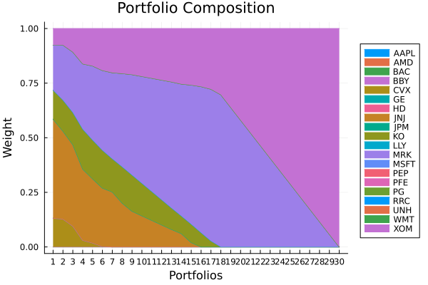
The efficient frontier is just a special case of a pareto front, we have a function that can plot pareto fronts and surfaces. We have to provide the weights and the prior. There are optional keyword parameters for the risk measure for the X-axis, Y-axis, Z-axis, and colourbar. Here we will use the Conditional Value at Risk as the X-axis, the arithmetic return, and the risk-return ratio as the colourbar.
# Risk-free rate of 4.2/100/252
plot_measures(res1.w, res1.pr; x = r, y = ExpectedReturn(; rt = res1.ret),
              c = ExpectedReturnRiskRatio(; rt = res1.ret, rk = r, rf = 4.2 / 100 / 252),
              title = "Efficient Frontier", xlabel = "CVaR", ylabel = "Arithmetic Return",
              colorbar_title = "\nRisk/Return Ratio", right_margin = 6Plots.mm)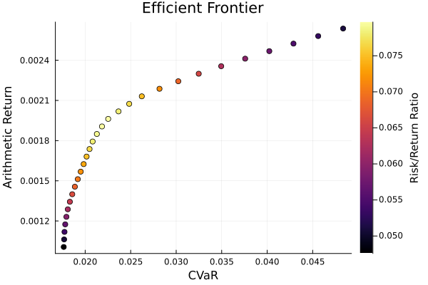
The plot_measures function can plot all sorts of pareto fronts. We can even use the ratio of two risk measures as the colourbar.
plot_measures(res1.w, res1.pr; x = r, y = ConditionalDrawdownatRisk(),
              c = RiskRatioRiskMeasure(; r1 = ConditionalDrawdownatRisk(), r2 = r),
              title = "Pareto Front", xlabel = "CVaR", ylabel = "CDaR",
              colorbar_title = "\nCDaR/CVaR Ratio", right_margin = 6Plots.mm)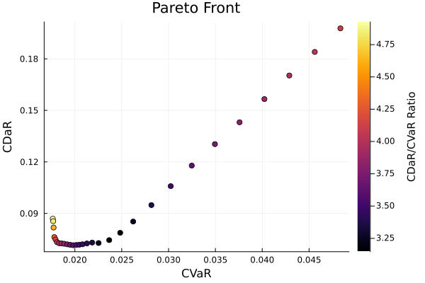
This page was generated using Literate.jl.